Recommendation systems drive engagement on many of the most popular online platforms. As the growth in the volume of data available to power these systems accelerates rapidly, data scientists are increasingly turning from more traditional machine learning methods to highly expressive deep learning models to improve the quality of their recommendations. Google’s Wide & Deep architecture has emerged as a popular choice of model for these problems, both for its robustness to signal sparsity, as well as its user-friendly implementation in TensorFlow via the DNNLinearCombinedClassifier API. While the cost and latency induced by the complexity of these deep learning models can be initially very expensive for inference applications, we’ll show that an accelerated, mixed-precision implementation of them optimized for NVIDIA GPUs can drastically reduce latency while obtaining impressive improvements in cost/inference. This paves the way for fast, low-cost, scalable recommendation systems well suited to both online and offline deployment and implemented using simple and familiar TensorFlow APIs.
In this blog, we describe a highly optimized, GPU-accelerated inference implementation of the Wide & Deep architecture based on TensorFlow’s DNNLinearCombinedClassifier API. The solution we propose allows for easy conversion from a trained TensorFlow Wide & Deep model to a mixed precision inference deployment. We also present performance results of this solution based on a representative dataset and show that GPU inference for Wide & Deep models can produce up to a 13x reduction in latency or a 11x throughput improvement in online and offline scenarios respectively.
Background
The Recommendation Problem
While we all likely have an intuitive understanding of what it is to make a recommendation, the question of how a machine learning model might make one is much less obvious. After all, there is something very prescriptive about the concept of a recommendation: “you should watch movie A”, “you should eat the tagliatelle at restaurant B”. How can a model know what I should do?
The answer is that, really, it doesn’t. Rather, we use machine learning to model the ways in which users interact with the relevant items. An interaction might mean a click on an ad, a play on a video, a purchase on a web-based store, a review on a restaurant, or any number of outcomes that our application might be interested in inducing. Machine learning models use data about previous interactions to forecast the likelihood of new interactions; we recommend the ones the model deems most likely to occur.
How the model makes these forecasts will depend on the type of data that you have. If you only have data about which interactions have occurred in the past, you’ll probably be interested in training collaborative filtering models via something like singular value decomposition or variational autoencoding. If you have data describing the entities that have interacted (e.g. a user’s age, the category of a restaurant’s cuisine, the average review for a movie), you can model the likelihood of a new interaction given these properties at the current moment.
Training vs. Inference
Broadly, the life-cycle of a machine learning model can be split into two phases. In the first, we train the model to make good forecasts by presenting it with examples of interactions (or non-interactions) between users and items from the past. Once it has learned to make predictions with a sufficient level of accuracy, we deploy the model as a service to infer the likelihood of new interactions.
Let’s take an example to make things more concrete. Say we have an app on which users find and rate restaurants, and we’d like to build a recommendation service to suggest new restaurants which users are likely to enjoy. We might train our model by presenting it with data about a user and data about a restaurant that was rated by that user, and ask it to score on a scale of 0-1 how likely it is that the user rated the restaurant higher than a 5 out of 10. We then show it the answer so that it can update itself in such a way that, after a few million iterations of guessing, its answers can get pretty good.
Once its education is complete, it’s time for our model to put that newly acquired skill to good use. It needs to get a job, but all it knows how to do is tell me whether or not a given user might enjoy a given restaurant. If what I’m interested in is finding new restaurants to show to users, that skill doesn’t seem particularly helpful, since if I knew which users and restaurants to pair together a priori, I wouldn’t need the model in the first place!
So we rephrase the problem: we pair a single user with hundreds or thousands of candidate restaurants, collect the likelihoods that the user enjoys each of them, and then show the user the restaurant they are rated most likely to enjoy. This inference stage utilizes a different pattern of data consumption than the one we saw during training, pairing one user up with many ads instead of one user with one ad, and so requires different design and data representation considerations.
The question of how to train these models efficiently is a rich and interesting problem in its own right, and is an area of active development for NVIDIA. However, we’ve often found that inference proves to be the more acute pain point for data scientists in the recommendation space. Deep learning models, though powerful, frequently require much more compute than their machine learning counterparts. This translates to higher latency (how long you have to wait for your recommendations) and lower throughput (how many recommendations you can make per second, which correlates with cost) when models are deployed for inference. If your highly skilled model takes too long to do its job, or costs too much, you might just abandon it altogether in lieu of something less skilled but faster and cheaper.
In addition to compute requirements, the inference stage also poses other system level considerations that play into the latency and throughput measurements of a deployment. The site at which the recommendation query is generated (say, your smartphone) typically does not have the compute capability to run a recommendation model in a reasonable amount of time. A standard way to solve this is to go to a client-server model where the client generates a recommendation query and sends it to a remote server that performs all the compute tasks pertaining to the model and send the results back to the client. This introduces a potential bottleneck as data needs to be sent over the network from the client to the server and back. To extract the highest value from a server, it is useful to have multiple clients send queries to a single server. This adds another layer of complexity in scheduling these client queries on the server optimally. Further, if the model is run on a GPU, data transfers to the GPU also play a role in performance. A recommendation deployment is more involved that just compute and a full system level analysis is imperative in understanding the end-to-end performance of the deployment.
Wide & Deep
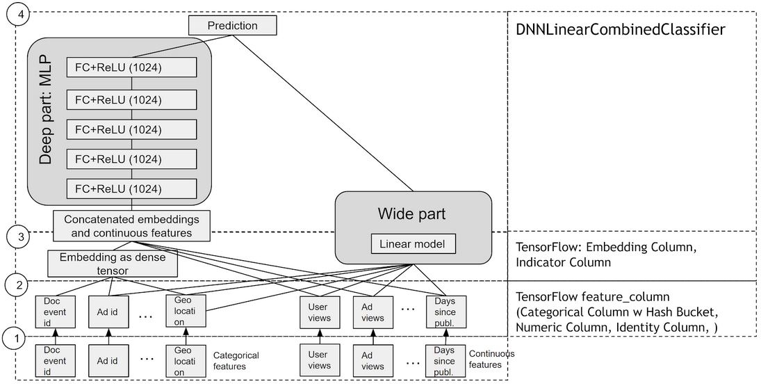
The principal components of a Wide & Deep network are a Dense Neural Network (DNN) and a linear model, whose outputs are summed to create an interaction probability. Categorical variables are embedded into continuous vector spaces before being fed to the DNN via learned or user-determined embeddings. What makes this model so successful for recommendation tasks is that it provides two avenues of learning patterns in the data, “deep” and “shallow”. The complex, nonlinear DNN is capable of learning rich representations of relationships in the data, but needs to see many examples of these relationships in order to do so well. The linear piece, on the other hand, is capable of “memorizing” simple relationships that may only occur a handful of times in the training set.
In combination, these two representation channels often end up providing more modelling power than either on its own. In Google’s original paper on the architecture, they reported statistically significant improvements in acquisition rates in their app store when using Wide & Deep versus a DNN or regression alone. NVIDIA has worked with many industry partners who reported improvements in offline and online metrics by using Wide & Deep as a replacement for more traditional machine learning models.
TensorFlow and DNNLinearCombinedClassifier
Now that we’ve decided we want to use a Wide & Deep model to make our recommendations, there arises the question of how to implement it. That is, how to define, in code, all the little mathematical functions that map from our raw data to the 0-1 prediction we’re looking for, not to mention all the calculus functions needed to define our updates and training procedure.
While there are many popular deep learning frameworks for implementing these models, we’ve chosen to focus on TensorFlow and in particular on its prebuilt implementation of Wide & Deep in its DNNLinearCombinedClassifier class, an instance of its Estimator API. We’ve chosen to direct our attention here not because it’s necessarily a better choice (although it does certainly offer powerful abstractions that make a data scientist’s job easier), but because of the ubiquity with which we see it being utilized in production scale recommendation systems at the major consumer internet companies we are fortunate enough to work with and learn from. Our hope is by working within the frameworks users are familiar and comfortable with, we can lower the barriers to implementing fast and scalable recommendation systems.
Dataset and Baseline Performance
The Outbrain Dataset
In order to explore how well GPUs could be suited to recommendation problems, we needed to find a dataset on which to benchmark our progress. This dataset not only needed to be representative of the sorts of problems we were seeing our customers work on, but needed to have the properties of a recommendation problem.
In particular, one of the key characteristics of a recommendation problem that we observed was a taxonomy of features: those belonging to a class describing the person or object to which we wish to make recommendations (the “requester”, so request features), and those belonging to a class describing those objects which we are considering recommending (the “items”, so item features).
Returning to our restaurant example from earlier, we might decide that a user’s age, location, and the categories of the last ten restaurants they used our app to find are relevant to informing which new restaurants they might like. Since these all describe the user who is requesting a restaurant recommendation, we would call these request features.
Likewise, we may decide that a restaurant’s average rating on our app, the category of its cuisine, and how long it’s been in business are relevant to whether a given user might enjoy it. Since these describe the restaurant (or item) that we’re considering recommending, we would call these “item features”.
As we discussed earlier, a large distinction between training and inference in the recommendation setting is that, during inference, we are generally interested in pairing the features from a single request with the features from many items, scoring the likelihood of interaction for each combination, and then selecting the item(s) with the highest likelihood of interaction.
What makes this distinction particularly important for inference performance is that these features, both request and item, often need to undergo some transformation from their raw representation to a representation digestible by neural networks. These transformations, defined in TensorFlow by feature columns, include nontrivial operations such as hashing, binning, vocabulary lookups, and embedding of categorical variables.
In a naive implementation, these transformations need to be computed for request features repeatedly for every item on which we wish to produce a recommendation. Moreover, if the model is being hosted on a dedicated remote inference server, we have to send copies of the request feature data for every item as well. This amounts to redundant compute and data I/O that can drastically reduce performance depending on the fraction of your features which belong to the request class. Therefore, it was important to us to find a dataset which possessed such a taxonomy in order to explore the effects of exploiting the invariance of request features across a batch of items.
This is obviously not the only consideration that makes a good choice of dataset. In order to ensure that we’d be tackling the right problems, we wanted a dataset whose features represented a robust but manageable sampling of the TensorFlow feature columns. Ideally, this dataset would also have clear, established inference benchmarks and an established target model accuracy (or equivalent metric) as a cherry on top.
Unfortunately, large public recommendation datasets are rare. Private companies are reticent about sharing internal datasets due to the difficulty of anonymizing data and the risk of sacrificing the competitive advantage that user interaction data provides. In the public sphere, the Netflix Prize and MovieLens datasets contain the wrong sort of data, primarily describing interactions between users and content, instead of describing their respective properties. The Criteo CTR dataset, while representing the latter type of data, has anonymized fields which can’t fit into the described feature taxonomy, and has only a handful of fields compared to the hundreds or even thousands we’ve observed in production use cases. Other alternatives like the Census Income dataset either can’t clearly be framed as a recommendation task, or, like the Criteo dataset, have too few features to adequately model performance on a real production application.
For our reference model, we used a subset of the features engineered by the 19th place finisher in the Kaggle ‘Outbrain Click Prediction Challenge’, in which competitors were tasked with predicting the likelihood with which a particular ad on a website’s display would be clicked-on. Competitors were given information about the user, display, document, and ad in order to train their models. More information can be found here. We chose this dataset for its size and more natural framing as a recommendation problem, as well as the sampling of feature columns it required.
While this dataset has many desirable properties, it still contained features that cannot be cleanly separated into one class or another. To simplify the inference workflow, we used a subset of the dataset which modeled these features as “idealized” recommendation features, features that describe only the requester or the items separately, but not any property which depends on both. We assume that any features whose names contain the words “ad”, “advertiser”, or “campaign” belong to the item class, and the rest are assumed to belong to the request class. We use the display_id feature to index request features, and the ad_id feature to index item features. This allows our dataset to fit more cleanly into a feature store model of data representation, where request and item features live in distinct data repositories, without having to muddy the waters with inference-time feature computation.
Out-of-the-box GPU Performance
What do we mean by model inference performance? When evaluating potential item candidates for the user, we do not measure database query and pre-filter (e.g. decision tree or manual logic) contribution. We do measure feature column preprocessing with the estimator, as well as copying inputs/results over the network.
There are two primary inference contexts:
- offline inference – pre-calculating the probabilities for many users at once
- online inference – making a real-time recommendation for a specific user
Therefore, we may be interested in optimizing three metrics:
- throughput, e.g. in users/second (offline)
- single inference latency (online)
- throughput while satisfying a set latency constraint
Our initial observation when using TensorFlow’s stock implementation was that not only were there redundancies in the request feature transformations as discussed above, but also that these transformations were implemented with dozens of ops inserted in the graph for small tasks like dimension expansion and in-range value checking. While these ops are computationally cheap in and of themselves, the overhead they introduce ends up bottlenecking performance, particularly on GPUs. Moreover, every feature has its own chain of tens to hundreds of ops for simple and essentially identical tasks like matrix lookups.
We removed this overhead by describing the intended logic in a concise config, which allows to implement ops in a fused, non-redundant, parallel fashion, while controlling execution precision.
Besides saving on redundant compute and network I/O, as we will see later, this implementation leverages the exceptional parallel computing power of NVIDIA GPUs to provide massive inference-time acceleration compared to native CPU-based implementations.
This acceleration unties the hands of the data scientist especially because it makes growing the model on the GPU easy while still meeting latency requirements. Moreover, in deployment, we see additional throughput coming from request-level parallelism.
How the Inference API Works
Using the API
While we’ll leave a detailed overview of the API to the notebooks, we’d like to draw attention to the key similarities and differences between our export process and the traditional TensorFlow Estimator export process, an overview of which can be found here.
Exporting a deep learning model typically requires specifying three components: the graph of operations that constitutes our model, the weights used to perform those operations, and the size and types of inputs that feed them. In the typical TensorFlow workflow, these components are defined by the feature columns describing the inputs and transformations, the Estimator which manages the weights, and its model function which describes the neural network graph (which is pre-defined for canned Estimators like the DNNLinearCombinedClassifier). The following lines from the export notebook are worth paraphrasing here, to highlight how this process works:
wide_columns, deep_columns = ...
estimator = tf.estimator.DNNLinearCombinedClassifier(
    linear_feature_columns=wide_columns,
    dnn_feature_columns=deep_columns,
    ...)

# infer input shapes and types from feature_columns as a parse_example_spec
parse_example_spec = \
    tf.feature_column.make_parse_example_spec(deep_columns + wide_columns)

# expose serialized Example protobuf string input and parse to feature tensors
# with a serving_input_receiver_fn
cpu_serving_input_receiver_fn = \
      tf.estimator.export.build_parsing_serving_input_receiver_fn(parse_example_spec)

# export in saved_model format
estimator.export_saved_model('/tmp', cpu_input_serving_receiver_fn)
| Listing 1: Pseudo-code for standard export of a TensorFlow Estimator |
Our API uses all the same information, in just about all the same ways, with a couple caveats. The first is that instead of mapping from serialized protobuf strings to feature tensors, our serving_input_receiver_fn maps from feature tensors to the dense vectors that get fed to the DNN. Unfortunately, the model function used by DNNLinearCombinedClassifier under the hood can’t accept these vectors, so we have built an almost exact copy of it which can (it’s a single line change) and swap it out.
The second caveat is that there is useful information about features from an optimization standpoint that isn’t contained in the feature columns. In particular, feature columns contain no information about the class to which a feature belongs (request or item), the benefits of which we’ve already discussed. They also don’t tell us whether a categorical feature is one-hot (can only take on a single category at a time, like a unique ID) or multi-hot (can take on many categories at a time, like describing a restaurant as “casual” and “Italian”). One-hot categoricals are just a special case of multi-hot, but knowing this information beforehand allows us to implement embedding lookups on GPUs efficiently and optimize memory allocation.
We provide the option of specifying this information via maps from feature names to flags indicating either request or item (0 or 1) or one-hot or multi-hot (1 or -1). These maps can come either as functions or dictionaries, as seen below:
# either functions
import re
AD_KEYWORDS = ['ad', 'advertiser', 'campain']
AD_REs = ['(^|_){}_'.format(kw) for kw in AD_KEYWORDS]
AD_RE = re.compile('|'.join(AD_REs))
level_map = lambda name: 0 if re.search(AD_RE, name) is None else 1

# or explicit dicts
from features import \
    REQUEST_SINGLE_HOT_COLUMNS, ITEM_SINGLE_HOT_COLUMNS, \
    REQUEST_MULTI_HOT_COLUMNS, ITEM_MULTI_HOT_COLUMNS
num_hot_map = {name: 1 for name in REQUEST_SINGLE_HOT_COLUMNS+ITEM_SINGLE_HOT_COLUMNS}
num_hot_map.update({name: -1 for name in REQUEST_MULTI_HOT_COLUMNS + ITEM_MULTI_HOT_COLUMNS})
| Listing 2: Mappings for specifying feature class and categorical properties |
If you’re not sure how your features fall into these camps, for each mapping there is always a more general case, so just leave it blank and we’ll assume that all your features are item level and multi-hot (for categoricals).
Once we’ve specified this extra information, the export process looks extremely similar:
from model import build_model_fn
from recommender_exporter import RecommenderExporter

wide_columns, deep_columns = ...
estimator = tf.estimator.DNNLinearCombinedClassifier(
    linear_feature_columns=wide_columns,
    dnn_feature_columns=deep_columns,
    ...)

# couple extra function calls
model_fn = build_model_fn(...)
exporter = RecommenderExporter(
    estimator, # for the weights
    deep_columns, # for the inputs and transformations
    wide_columns,
    model_fn, # for the graph
    level_map, # for request vs. item
    num_hot_map, # for one vs. multi -hot
    wide_combiner=...)

# then the same
gpu_input_serving_receiver_fn = exporter.get_input_serving_receiver_fn()
estimator.export_saved_model('/tmp', gpu_input_serving_receiver_fn)
| Listing 3: Pseudo-code for GPU-accelerated model export |
This will export a TensorFlow Saved Model with our accelerated lookup op inserted into the graph. While we can serve and make calls to this Saved Model, the API isn’t as neat due to the vectorized input that the graph expects, and still incurs overhead from TensorFlow. To accelerate the graph further as TensorRT executable engine, we need only freeze the Saved Model into a TensorFlow GraphDef, which TensorFlow has built-in utilities for, and then leverage our provided conversion script, which uses information encoded in the graph def to compile our TensorRT engine. See the notebook for examples on how this achieved with a simple Flask app.
End-to-end, our export pipeline looks like this:
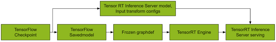
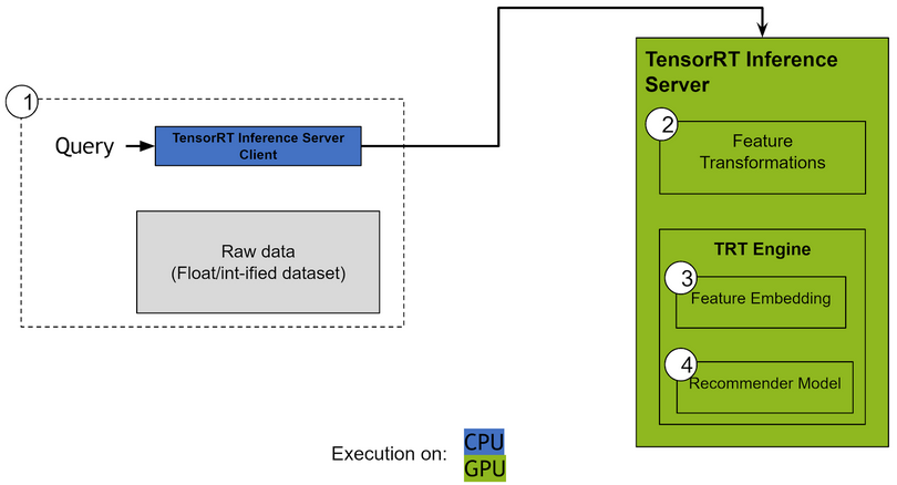
There are two ways to deploy the converted model. First, if the inference can happen locally (same server as where the request comes from), we can skip NVIDIA Triton Inference Server and use the custom class with CUDA and TensorRT parts. Second, for remote inference or ease-of-use, Triton Server uses custom backend for both custom CUDA code and TensorRT engine inference.
Performance Breakdown
Our code supports both local and remote inference. While direct local inference can yield the best latency and CPU utilization, this requires meticulous tuning. Remote inferencing is more flexible since it decouples query generation and the inference computation. Triton Server is a solution for remote inferencing and allows easy optimization to fully utilize the compute capability available. This is done at many levels, scheduling incoming queries, pipeline optimization by hosting multiple copies of the model served on a GPU, node level optimization to efficiently utilize all available GPUs and more. It makes transition to remote inference seamless, which helps with using common node configurations. Its perf_client test utility helps vary the client concurrency to issue multiple concurrent queries to the server instance and measure throughput and latency. Here we present throughput-optimized and latency optimized data for our model obtained by testing with the aforementioned features.
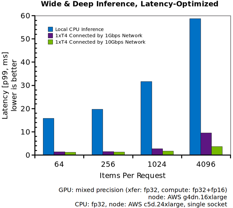
In a remote inference scenario, generated queries need to be communicated to a remote server. This is not typically a bottleneck when the amount of data transferred is small and the compute requirement is large. However, Wide & Deep models can consume lots of features into few MLP layers. As a result, the amount of data transferred is larger and the compute required is smaller causing the network bandwidth to have an effect on observed end-to-end performance. This is exaggerated when the compute is heavily accelerated on GPUs. For our model tested here, a 1Gbps network between the client and server bottlenecks performance at larger items per request and moving to a 10Gbps effectively removes that bottleneck.
The figure below shows the p99 latency for a query as a function of the items per request for the model run on a CPU compared to the model run on an NVIDIA T4 GPU. The GPU runs use the client-server model where the client and servers are placed on different nodes connected by either a 1Gbps or a 10Gbps network. The CPU runs are performed locally without any network bottlenecks. The CPU chosen here is a single Xeon Platinum 8275CL with 24 cores and 48 threads (available on a c5d.24xlarge AWS instance). Each query is split and parallelized across all cores of the CPU. We use either the official TensorFlow container or Intel’s TensorFlow container to measure the CPU performance based on which is faster. For the GPU runs, each query is processed unsplit on a single NVIDIA T4 GPU with the Triton Server parameters optimized for latency. The plot shows that the GPU latency is more than an order of magnitude lower than the CPU latency when many items are paired with a single request. At 4,096 items per request, the CPU latency is ~55ms while the GPU latency is ~8ms on a 1Gbps network or ~4ms on a 10 Gbps network. Even at lower items per request, the GPU has vastly lower latency with ~1.2ms compared to ~15ms for the CPU at 64 items per request.
If latency constraints are not important, like in offline processing, then we can choose Triton Server parameters to optimize throughput instead. The figure below shows the throughput as a function of items per request for a throughput optimized configuration of the model. Like in the latency optimized case, the network bandwidth between the client and server affects performance. At the lowest items per request, there is not enough work to saturate the GPU. As the items per request increases to 256, we see better throughput since the GPU is more efficient. As we increase the items per request even further, the amount of work required increases linearly and the throughput achieved drops correspondingly.

| Items per request | Latency optimized | Throughput optimized | ||
| Latency | Throughput | Latency | Throughput | |
| 64 | 13.1x | 12.8x | 10.7x | 3.7x |
| 256 | 14.9x | 14.7x | 42.4x | 6.5x |
| 1,024 | 18.0x | 17.6x | 93.2x | 11.5x |
| 4,096 | 15.9x | 15.0x | 139.5x | 9.4x |
| Table 1: Improvement in latency and throughput of GPU over CPU. The numbers here correspond to the CPU and the 10Gbps GPU runs. |
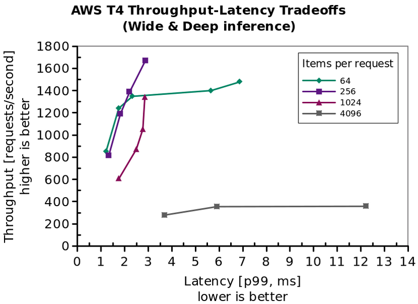
To demonstrate throughput optimization under latency constraint, we sweep through client and server concurrency (that is, how many requests does a client wait on concurrently, and how many models does a server allow to run in parallel), and select the configurations that make useful tradeoffs. The figure below shows these throughput-latency tradeoff curves for different items per request. As you increase the client and server concurrency, the throughput increases until the GPU is saturated with work. After this, the latency increases substantially with only a small throughput increase.
Why does it run so fast?
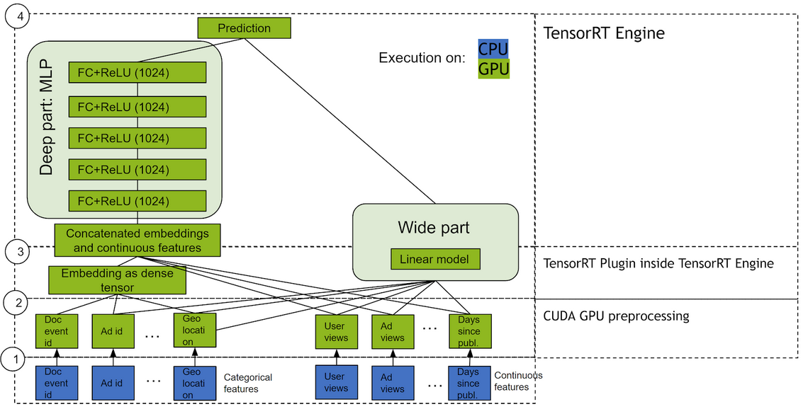
GPU Preprocessing for TensorFlow feature_columns and Fused Embedding Lookups
First, the data is preprocessed in TensorFlow feature columns. Thinking of Extract-Transform-Load, we leave the Extract to the user (with a sample CSV implementation), Transform in the feature columns, but after already having Loaded the tensors into the GPU in an optimized fashion. In order to leverage high integer instruction throughput on GPU we reorder the concatenations for best performance, and port the hashing to CUDA. CUDA made it very easy to vectorize arbitrary code using a simple wrapper function around the CPU hashing implementation. We fuse the whole (int|float) → string → hash → hash_bucket chain into a single kernel.
Late into the feature columns, embeddings are looked up using indices obtained above. We export the feature columns with a config that allows for GPU parallelization. GPUs have a higher memory bandwidth, which defines embedding performance given optimal software that utilizes ability to schedule different kinds of instructions in parallel.
Accelerated Matrix Multiplies for the MLP
Last but not least, the embeddings feed into a Multilayer Perceptron (MLP) that is part of the deep portion of the model. It’s the most compute intensive part of Wide & Deep models. For batched computations, the MLP is essentially a sequence of matrix multiplications with activations and other pointwise operations like batch normalization between them. Matrix multiplications require much more math operations (that scale cubically) compared to memory operations (that scale quadratically). Since GPUs are designed to provide much larger compute throughput, matrix multiplies typically see a tremendous performance boost when run in a highly parallel fashion on a GPU. Additionally, Volta and Turing architectures of NVIDIA GPUs, have Tensor Cores which further accelerate matrix multiplies when run in mixed or reduced precision.
NVIDIA GPUs have the architectural features to make MLP computations very fast. To leverage these architectural features and get the highest performance, the software stack plays a pivotal role. We use NVIDIA TensorRT, a platform for high performance deep learning inference on NVIDIA GPUs. TensorRT performs graph level optimization and architecture specific optimization to generate a TensorRT engine that executes the graph in a highly performant manner. TensorRT’s optimization selects the right GPU kernels for the matrix multiplies based on the size of the matrices and the GPU architecture being used. TensorRT also enables using mixed and reduced precision to leverage Tensor Cores. Memory bandwidth is an increasingly growing source of bottlenecks in many applications since compute throughput is typically much larger than the memory bandwidth on most architectures. TensorRT has powerful optimization techniques to perform kernel fusion that improves memory locality for computing activation functions and pointwise kernels and further speeds up the pipeline.
API Flexibility and Constraints
There are design elements in our API that are worth highlighting beyond the drastic improvements in actual model compute time. First, unlike other attempts to accelerate Wide & Deep models that align all the categorical embedding sizes in order to treat the entire deep embedding step as a single multi-hot lookup, we make no assumptions about the relative sizes of your embeddings. This allows data scientists to freely hyperparameter search over the space of embedding sizes without having to worry about inference time performance. There is no need to pre-transform features and store them, as the transformation method may change with the model cadence. This saves on storage cost while maintaining the original model representation. Doing it live on the CPU would create a bottleneck of its own.
While we still have many feature column types for which to add support, we try to make as few assumptions as we can about your data for those that we do. While considerations should be made about how engineered features will impact inference performance, such considerations should never preclude a data scientist from being able to exploit a useful feature.
A notable exception to this rule is our lack of support for string data, which we elected to exclude under the assumption that, for most use cases, string data can be converted to an integer index before storage without significant loss of generality or abstraction. This not only reduces storage costs and CPU load during preprocessing, but reduces network traffic in dedicated inference server settings. While our dataset does not include strings, if our assumptions about “int-ification” are misguided, we would welcome that feedback.
There are instances where we do ask the user to provide assumptions about their data. These include the arguments avg_nnz_per_feature and items_per_request needed for the compilation of the TensorRT engine. The former could prove problematic in use cases where the number of indices in a multi-hot categorical feature can vary by orders of magnitude from one example to the next, or where the max number of indices to expect cannot be known beforehand. The latter constraint faces similar issues for situations where candidate items come from upstream filters whose number of candidates can’t be known beforehand (though there are feasible workarounds in this case).
The final API feature to highlight is that through introducing the specification of nnz values for multi-hot features, we make unnecessary the SparseTensor machinery that TensorFlow leverages in its parse_example op. This, by extension, largely obviates the need for tf.Example protobufs as an input representation to the network, saving time and compute on the tautology of building, serializing, then immediately deserializing data which you already have.
Moreover, in conjunction with our Triton Server custom backend plugin, this means users can map directly from raw data representations to recommendation scores with negligible overhead. Such data representations enable more robust abstraction all while offering substantially higher performance.
Looking Forward
Right now, our support of TensorFlow feature column types extends only to those which were required by the Outbrain dataset. To reiterate, those are numeric columns with shape=(1,), for scalar-valued numeric features; categorical_column_with_identity, categorical_column_with_hash_bucket, and embedding and indicator columns to wrap them in. Our priority is to extend support to the remaining feature columns, with the top of our list being
- Crossed columns
- Vector-valued numeric columns (
len(shape) == 1andshape[0] > 1) categorical_column_with_vocabulary_list(for integer vocabularies)bucketized_columnweighted_categorical_column
In a field marked by the diversity of its problems, we’re sure that more functionality will be needed in order to adequately address the use cases of our users. Filing Github issues on this repo would be a great way to suggest novel functionality or to help reprioritize the roadmap given above.
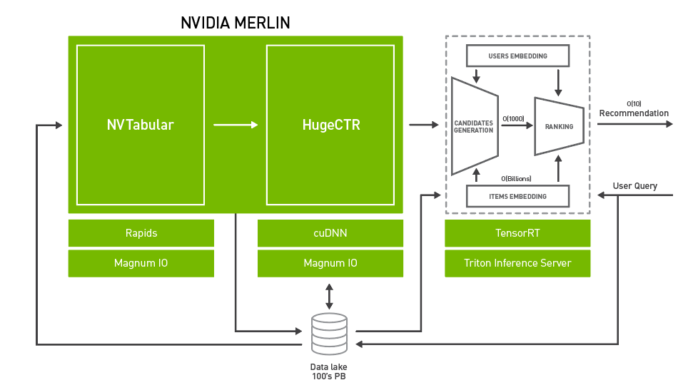
NVIDIA is also working on accelerating other parts of the recommender pipeline. Data ingestion and pre-processing (ETL) is a major component of the recommender system pipeline and RAPIDS can be leveraged to accelerate those components on GPU. If you haven’t already, take a look at our work on accelerating recommender system training using Rapids and PyTorch for RecSys 2019 challenge. Another parallel effort to train recommender systems with large embedding tables on multiple GPUs is also under active development, you can check it out here: https://github.com/NVIDIA/HugeCTR
Conclusion
In this article we demonstrated how to get at least a 10x reduction in latency with about 13x more throughput for recommenders using GPUs. Such incredible speed-up will help reduce deployment costs of serving live inference for recommender systems. Learn more about our work by signing up at the early access page and try the interactive ipython notebook demos to convert and deploy your TensorFlow Wide & Deep model for inference. Use the comments below to tell us how you plan to adopt and extend this project.