
Deep learning is revolutionizing the way that industries are delivering products and services. These services include object detection, classification, and segmentation for computer vision, and text extraction, classification, and summarization for language-based applications. These applications must run in real time.
Most of the models are trained in floating-point 32-bit arithmetic to take advantage of a wider dynamic range. However, at inference, these models may take a longer time to predict results compared to reduced precision inference, causing some delay in the real-time responses, and affecting the user experience.
It’s better in many cases to use reduced precision or 8-bit integer numbers. The challenge is that simply rounding the weights after training may result in a lower accuracy model, especially if the weights have a wide dynamic range. This post provides a simple introduction to quantization-aware training (QAT), and how to implement fake-quantization during training, and perform inference with NVIDIA TensorRT 8.0.
Overview
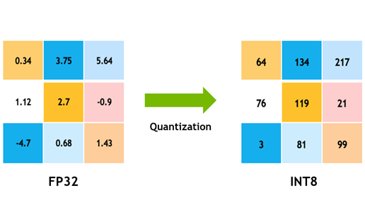
Model quantization is a popular deep learning optimization method in which model data—both network parameters and activations—are converted from a floating-point representation to a lower-precision representation, typically using 8-bit integers. This has several benefits:
- When processing 8-bit integer data, NVIDIA GPUs employ the faster and cheaper 8-bit Tensor Cores to compute convolution and matrix-multiplication operations. This yields more compute throughput, which is particularly effective on compute-limited layers.
- Moving data from memory to computing elements (streaming multiprocessors in NVIDIA GPUs) takes time and energy, and also produces heat. Reducing the precision of activation and parameter data from 32-bit floats to 8-bit integers results in 4x data reduction, which saves power and reduces the produced heat.
- Some layers are bandwidth-bound (memory-limited). That means that their implementation spends most of its time reading and writing data, and therefore reducing their computation time does not reduce their overall runtime. Bandwidth-bound layers benefit most from reduced bandwidth requirements.
- A reduced memory footprint means that the model requires less storage space, parameter updates are smaller, cache utilization is higher, and so on.
Quantization methods
Quantization has many benefits but the reduction in the precision of the parameters and data can easily hurt a model’s task accuracy. Consider that 32-bit floating-point can represent roughly 4 billion numbers in the interval [-3.4e38, 3.40e38]. This interval of representable numbers is also known as the dynamic-range. The distance between two neighboring representable numbers is the precision of the representation.
Floating-point numbers are distributed nonuniformly in the dynamic range and about half of the representable floating-point numbers are in the interval [-1,1]. In other words, representable numbers in the [-1, 1] interval would have higher precision than numbers in [1, 2]. The high density of representable 32-bit floating-point numbers in [-1, 1] is helpful in deep learning models where parameters and data have most of their distribution mass around zero.
Using an 8-bit integer representation, however, you can represent only 28 different values. These 256 values can be distributed uniformly or nonuniformly, for example, for higher precision around zero. All mainstream, deep-learning hardware and software chooses to use a uniform representation because it enables computing using high-throughput parallel or vectorized integer math pipelines.
To convert the representation of a floating-point tensor (


This is symmetric quantization because the dynamic-range is symmetric about the origin. 

At the top of Figure 1 is a diagram of an arbitrary floating-point tensor 


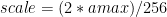
The method shown here to compute the scale uses the full range that you can represent with signed 8-bit integers: [-128, 127]. TensorRT Explicit Precision (Q/DQ) networks use this range when quantizing weights and activations.
There is tension between the dynamic range chosen to represent using 8-bit integers and the error introduced by the rounding operation. A larger dynamic range means that more values from the original floating-point tensor get represented in the quantized tensor, but it also means using a lower precision and introducing a larger rounding error.
Choosing a smaller dynamic range reduces the rounding error but introduce a clipping error. Floating-point values that are outside the dynamic range are clipped to the min/max value of the dynamic range.
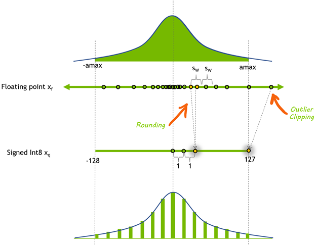 . The symmetric dynamic range of
 ![x_{f} [-amax, amax]](https://s0.wp.com/latex.php?latex=x_%7Bf%7D+%5B-amax%2C+amax%5D&bg=transparent&fg=000&s=0&c=20201002) is mapped through quantization to [-128, 127].
is mapped through quantization to [-128, 127].To address the effects of the loss of precision on the task accuracy, various quantization techniques have been developed. These techniques can be classified as belonging to one of two categories: post-training quantization (PTQ) or quantization-aware training (QAT).
As the name suggests, PTQ is performed after a high-precision model has been trained. With PTQ, quantizing the weights is easy. You have access to the weight tensors and can measure their distributions. Quantizing the activations is more challenging because the activation distributions must be measured using real input data.
To do this, the trained floating-point model is evaluated using a small dataset representative of the task’s real input data, and statistics about the interlayer activation distributions are collected. As a final step, the quantization scales of the model’s activation tensors are determined using one of several optimization objectives. This process is calibration and the representative dataset used is the calibration-dataset.
Sometimes PTQ is not able to achieve acceptable task accuracy. This is when you might consider using QAT. The idea behind QAT is simple: you can improve the accuracy of quantized models if you include the quantization error in the training phase. It enables the network to adapt to the quantized weights and activations.
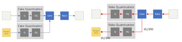
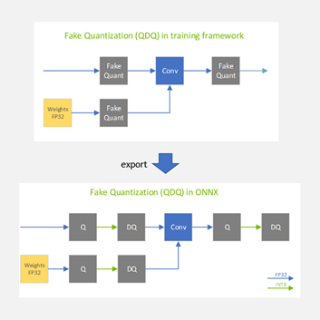
There are various recipes to perform QAT, from starting with an untrained model to starting with a pretrained model. All recipes change the training regimen to include the quantization error in the training loss by inserting fake-quantization operations into the training graph to simulate the quantization of data and parameters. These operations are called ‘fake’ because they quantize the data, but then immediately dequantize the data so the operation’s compute remains in float-point precision. This trick adds quantization noise without changing much in the deep-learning framework.
In the forward-pass, you fake-quantize the floating-point weights and activations and use these fake-quantized weights and activations to perform the layer’s operation. In the backward pass, you use the weights’ gradients to update the floating-point weights. To deal with the quantization gradient, which is zero almost everywhere except for points where it is undefined, you use the (straight-through estimator (STE), which passes the gradient as-is through the fake-quantization operator. When the QAT process is done, the fake-quantization layers hold the quantization scales that you use to quantize the weights and activations that the model is used for inference.
PTQ is the more popular method of the two because it is simple and doesn’t involve the training pipeline, which also makes it the faster method. However, QAT almost always produces better accuracy, and sometimes this is the only acceptable method.
Quantization in TensorRT
TensorRT 8.0 supports INT8 models using two different processing modes. The first processing mode uses the TensorRT tensor dynamic-range API and also uses INT8 precision (8-bit signed integer) compute and data opportunistically to optimize inference latency.
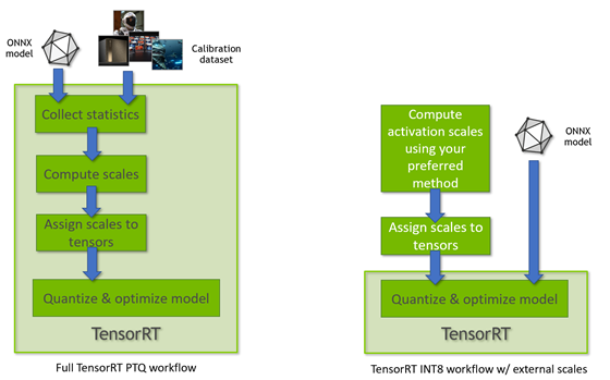
This mode is used when TensorRT performs the full PTQ calibration recipe and when TensorRT uses preconfigured tensor dynamic-ranges (Figure 3). The other TensorRT INT8 processing mode is used when processing floating-point ONNX networks with QuantizeLayer/DequantizeLayer layers and follows explicit quantization rules. For more information about the differences, see Explicit-Quantization vs. PTQ-Processing in the TensorRT Developer Guide.
TensorRT Quantization Toolkit
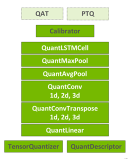
The TensorRT Quantization Toolkit for PyTorch compliments TensorRT by providing a convenient PyTorch library that helps produce optimizable QAT models. The toolkit provides an API to automatically or manually prepare a model for QAT or PTQ.
At the core of the API is the TensorQuantizer module, which can quantize, fake-quantize, or collect statistics on a tensor. It is used together with QuantDescriptor, which describes how a tensor should be quantized. Layered on top of TensorQuantizer are quantized modules that are designed as drop-in replacements of PyTorch’s full-precision modules. These are convenience modules that use TensorQuantizer to fake-quantize or collect statistics on a module’s weights and inputs.
The API supports the automatic conversion of PyTorch modules to their quantized versions. Conversion can also be done manually using the API, which allows for partial quantization in cases where you don’t want to quantize all modules. For example, some layers may be more sensitive to quantization and leaving them unquantized improves task accuracy.
The TensorRT-specific recipe for QAT is described in detail in NVIDIA Quantization whitepaper, which includes a more rigorous discussion of the quantization methods and results from experiments comparing QAT and PTQ on various learning tasks.
Code example walkthrough
This section describes the classification-task quantization example included with the toolkit.
The recommended toolkit recipe for QAT calls for starting with a pretrained model, as it’s been shown that starting from a pretrained model and fine-tuning leads to better accuracy and requires significantly fewer iterations. In this case, you load a pretrained ResNet50 model. The command-line arguments for running the example from the bash shell:
python3 classification_flow.py --data-dir [path to ImageNet DS] --out-dir . --num-finetune-epochs 1 --evaluate-onnx --pretrained --calibrator=histogram --model resnet50_res
The --data-dir argument points to the ImageNet (ILSVRC2012) dataset, which you must download separately. The --calibrator=histogram argument specifies that the model should be calibrated, using the histogram calibrator, before fine-tuning the model. The rest of the arguments, and many more, are documented in the example.
The ResNet50 model is originally from Facebook’s Torchvision package, but because it includes some important changes (quantization of skip-connections), the network definition is included with the toolkit (resnet50_res). For more information, see Q/DQ Layer-Placement Recommendations.
Here’s a brief overview of the code. For more information, see Quantizing ResNet50.
 # Prepare the pretrained model and data loaders
 model, data_loader_train, data_loader_test, data_loader_onnx = prepare_model(
         args.model_name,
         args.data_dir,
         not args.disable_pcq,
         args.batch_size_train,
         args.batch_size_test,
         args.batch_size_onnx,
         args.calibrator,
         args.pretrained,
         args.ckpt_path,
         args.ckpt_url)
The function prepare_model instantiates the data loaders and model as usual, but it also configures the quantization descriptors. Here’s an example:
 # Initialize quantization
 if per_channel_quantization:
         quant_desc_input = QuantDescriptor(calib_method=calibrator)
 else:
         quant_desc_input = QuantDescriptor(calib_method=calibrator, axis=None)
 quant_nn.QuantConv2d.set_default_quant_desc_input(quant_desc_input)
 quant_nn.QuantConvTranspose2d.set_default_quant_desc_input(quant_desc_input)
 quant_nn.QuantLinear.set_default_quant_desc_input(quant_desc_input)
 quant_desc_weight = QuantDescriptor(calib_method=calibrator, axis=None)
 quant_nn.QuantConv2d.set_default_quant_desc_weight(quant_desc_weight)
 quant_nn.QuantConvTranspose2d.set_default_quant_desc_weight(quant_desc_weight)
 quant_nn.QuantLinear.set_default_quant_desc_weight(quant_desc_weight)
Instances of QuantDescriptor describe how to calibrate and quantize tensors by configuring the calibration method and axis of quantization. For each quantized operation (such as quant_nn.QuantConv2d), you configure the activations and weights in QuantDescriptor separately because they use different fake-quantization nodes.
You then add fake-quantization nodes in the training graph. The following code (quant_modules.initialize) dynamically patches PyTorch code behind the scenes so that some of the torch.nn.module subclasses are replaced by their quantized counterparts, instantiates the model’s modules, and then reverts the dynamic patch (quant_modules.deactivate). For example, torch.nn.conv2d is replaced by pytorch_quantization.nn.QuantConv2d, which performs fake-quantization before performing the 2D convolution. The method quant_modules.initialize should be invoked before model instantiation.
quant_modules.initialize()
model = torchvision.models.__dict__[model_name](pretrained=pretrained)
quant_modules.deactivate()
Next, you collect statistics (collect_stats) on the calibration data: feed calibration data to the model and collect activation distribution statistics in the form of a histogram for each layer to quantize. After you’ve collected the histogram data, calibrate the scales (calibrate_model) using one or more calibration algorithms (compute_amax).
During calibration, try to determine the quantization scale of each layer, so that it optimizes some objective, such as the model accuracy. There are currently two calibrator classes:
pytorch_quantization.calib.histogram—Uses entropy minimization (KLD), mean-square error minimization (MSE), or a percentile metric method (choose the dynamic-range such that a specified percentage of the distribution is represented).pytorch_quantization.calib.max—Calibrates using the maximum activation value (represents the entire dynamic range of the floating point data).
To determine the quality of the calibration method afterward, evaluate the model accuracy on your dataset. The toolkit makes it easy to compare the results of the four different calibration methods to discover the best method for a specific model. The toolkit can be extended with proprietary calibration algorithms. For more information, see the ResNet50 example notebook.
If the model’s accuracy is satisfactory, you don’t have to proceed with QAT. You can export to ONNX and be done. That would be the PTQ recipe. TensorRT is given the ONNX model that has Q/DQ operators with quantization scales, and it optimizes the model for inference. So, this is a PTQ workflow that results in a Q/DQ ONNX model.
To continue to the QAT phase, choose the best calibrated, quantized model. Use QAT to fine-tune for around 10% of the original training schedule with an annealing learning-rate schedule, and finally export to ONNX. For more information, see the Integer Quantization for Deep Learning Inference: Principles and Empirical Evaluation whitepaper.
There are a couple of things to keep in mind when exporting to ONNX:
- Per-channel quantization (PCQ) was introduced in ONNX opset 13, so if you are using PCQ as recommended, mind the opset version that you are using.
- The argument
do_constant_foldingshould be set to True to produce smaller models that are more readable.
torch.onnx.export(model, dummy_input, onnx_filename, verbose=False, opset_version=opset_version, do_constant_folding=True)
When the model is finally exported to ONNX, the fake-quantization nodes are exported to ONNX as two separate ONNX operators: QuantizeLinear and DequantizeLinear (shown in Figure 5 as Q and DQ).
QAT inference phase
At a high level, TensorRT processes ONNX models with Q/DQ operators similarly to how TensorRT processes any other ONNX model:
- TensorRT imports an ONNX model containing Q/DQ operations.
- It performs a set of optimizations that are dedicated to Q/DQ processing.
- It continues to perform the general optimization passes.
- It builds a platform-specific, execution-plan file for inference execution. This plan file contains quantized operations and weights.
Building Q/DQ networks in TensorRT does not require any special builder configuration, aside from enabling INT8, because it is automatically enabled when Q/DQ layers are detected in the network. The minimal command to build a Q/DQ network using the TensorRT sample application trtexec is as follows:
$ trtexec -int8 <onnx file>
TensorRT optimizes Q/DQ networks using a special mode referred to as explicit quantization, which is motivated by the requirements for network processing-predictability and control over the arithmetic precision used for network operation. Processing-predictability is the promise to maintain the arithmetic precision of the original model. The idea is that Q/DQ layers specify where precision transitions must happen and that all optimizations must preserve the arithmetic semantics of the original ONNX model.
Contrasting TensorRT Q/DQ processing and plain TensorRT INT8 processing helps explain this better. In plain TensorRT, INT8 network tensors are assigned quantization scales, using the dynamic range API or through a calibration process. TensorRT treats the model as a floating-point model when applying the backend optimizations and uses INT8 as another tool to optimize layer execution time. If a layer runs faster in INT8, then it is configured to use INT8. Otherwise, FP32 or FP16 is used, whichever is faster. In this mode, TensorRT is optimizing for latency only, and you have little control over which operations are quantized.
In contrast, in explicit quantization, Q/DQ layers specify where precision transitions must happen. The optimizer is not allowed to perform precision-conversions not dictated by the network. This is true even if such conversions increase layer precision (for example, choosing an FP16 implementation over an INT8 implementation) and even if such conversion results in a plan file that executes faster (for example, preferring INT8 over FP16 on V100 where INT8 is not accelerated by Tensor Cores).
In explicit quantization, you have full control over precision transitions and the quantization is predictable. TensorRT still optimizes for performance but under the constraint of maintaining the original model’s arithmetic precision. Using the dynamic-range API on Q/DQ networks is not supported.
The explicit quantization optimization passes operate in three phases:
- First, the optimizer tries to maximize the model’s INT8 data and compute using Q/DQ layer propagation. Q/DQ propagation is a set of rules specifying how Q/DQ layers can migrate in the network. For example,
QuantizeLayercan migrate toward the beginning of the network by swapping places with a ReLU activation layer. By doing so, the input and output activations of the ReLU layer are reduced to INT8 precision and the bandwidth requirement is reduced by 4x. - Then, the optimizer fuses layers to create quantized operations that operate on INT8 inputs and use INT8 math pipelines. For example,
QuantizeLayercan fuse withConvolutionLayer. - Finally, the TensorRT auto-tuner optimizer searches for the fastest implementation of each layer that also respects the layer’s specified input and output precision.
For more information about the main explicit quantization optimizations that TensorRT performs, see the TensorRT Developer Guide.
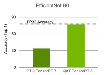
The plan file created from building a TensorRT Q/DQ network contains quantized weights and operations and is ready to deploy. EfficientNet is one of the networks that requires QAT to maintain accuracy. The following chart compares PTQ to QAT.
For more information, see the EfficientNet Quantization example on NVIDIA DeepLearningExamples.
Conclusion
In this post, we briefly introduced basic quantization concepts and TensorRT’s quantization toolkit and then reviewed how TensorRT 8.0 processes Q/DQ networks. We did a quick walkthrough of the ResNet50 QAT example provided with the Quantization Toolkit.
ResNet50 can be quantized using PTQ and doesn’t require QAT. EfficientNet, however, requires QAT to maintain accuracy. The EfficientNet B0 baseline floating-point Top1 accuracy is 77.4, while its PTQ Top1 accuracy is 33.9 and its QAT Top1 accuracy is 76.8.
For more information, see the GTC 2021 session, Quantization Aware Training in PyTorch with TensorRT 8.0.