In part 1, I introduced the code for profiling, covered the basic ideas of analysis-driven optimization (ADO), and got you started with the Nsight Compute profiler. In part 2, you apply what you learned to improve the performance of the code and then continue the analysis and optimization process.
Refactoring
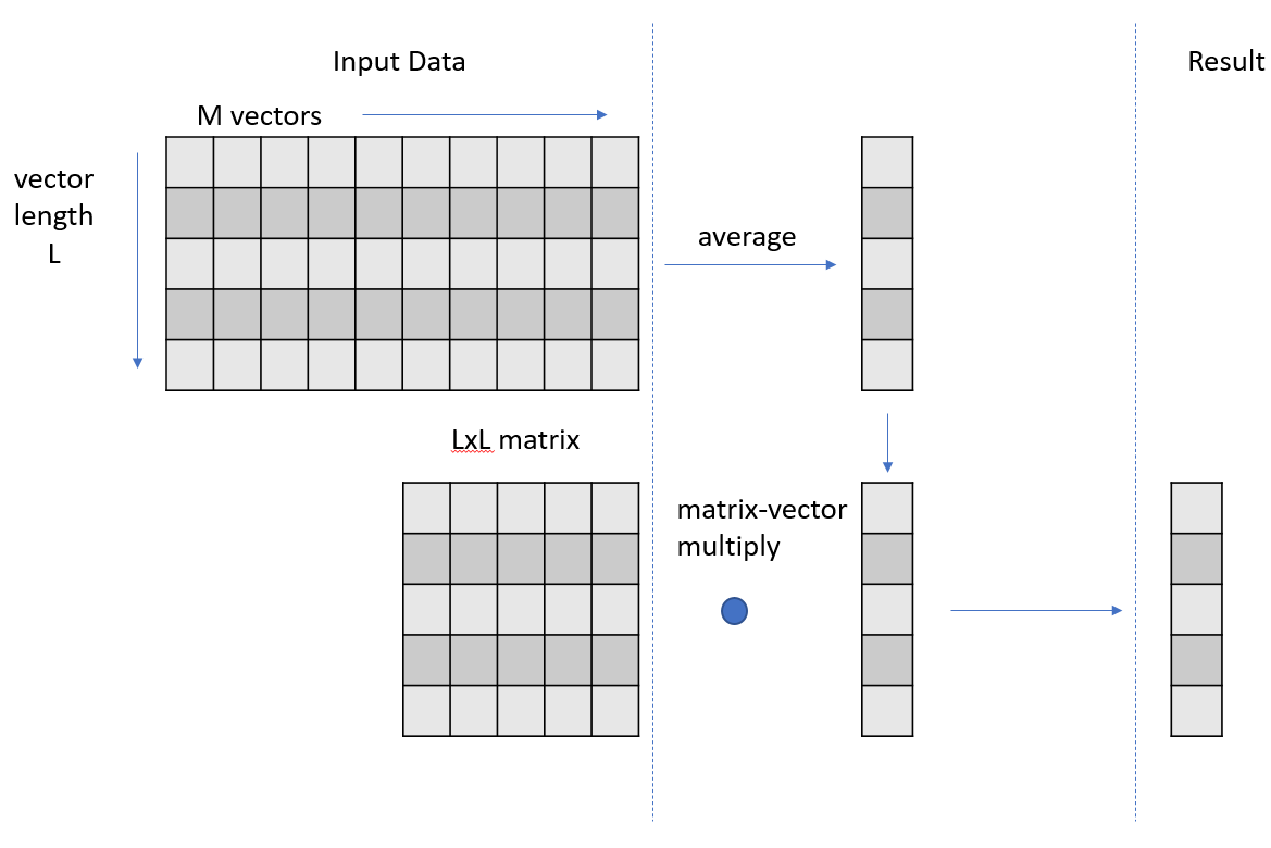
To refactor the code based on the previous analysis in part 1, you observe that your kernel design and the original CPU code has an outer loop that iterates over the N data sets. This means you are using one block to compute the results for all N data sets. Because the data sets are all independent, you can easily distribute this work across N blocks, and the code refactoring at this point is simple. Get rid of the outer loop, compute or replace the loop variable k using the blockIdx.x built-in variable, and then launch the kernel with N blocks instead of one block. Create a new version of your kernel code:
template
__global__ void gpu_version2(const T * __restrict__ input, T * __restrict__ output, const T * __restrict__ matrix, const int L, const int M, const int N){
  // parallelize threadIdx.x over vector length, and blockIdx.x across k (N)
  __shared__ T smem[my_L];
  int idx = threadIdx.x;
  int k = blockIdx.x;
    T v1 = 0;
    for (int i = 0; i < M; i++)  // perform vector averaging
      v1 += input[k*M*L+idx*M+i];
    v1 /= M;
    for (int i = 0; i < L; i++){ // perform matrix-vector multiply
      __syncthreads();
      smem[threadIdx.x] = v1 * matrix[i*L+idx];
      for (int s = blockDim.x>>1; s > 0; s>>=1){
        __syncthreads();
        if (threadIdx.x < s) smem[threadIdx.x] += smem[threadIdx.x+s];}
      if (!threadIdx.x) output[k+i*N] = smem[0];}
}
You also need to update the kernel launch:
gpu_version2<<<N, L>>>(d_input, d_output, d_matrix, L, M, N);
From this point forward, you should not have trouble with profiling due to extended profiling overhead, so you can restore the N value to its original value:
const int my_N = 1024;
If you recompile and run the code, you should now see something like the following results:
CPU execution time: 0.554662s
Kernel execution time: 0.07894s
|
|
baseline |
Step 1 |
|
Kernel duration: |
2.92s |
0.0789s |
That change has made a tremendous improvement in GPU performance. To continue the ADO process, you must start again with the profiler. Disconnect from the previous session, connect to a new session, and then launch again. Alternatively, because you are using Auto Profile, and there is only one kernel, you could also choose Resume instead of Run to Next Kernel, which would profile the rest of the application until it terminates.
After launching, you should not have to make any setting changes at this point. Choose Run to Next Kernel again. After about 10 seconds, a new results tab opens, labelled Untitled Y. Your previous results are still there, in the Untitled X tab, where X and Y are numbers like 1 and 2.
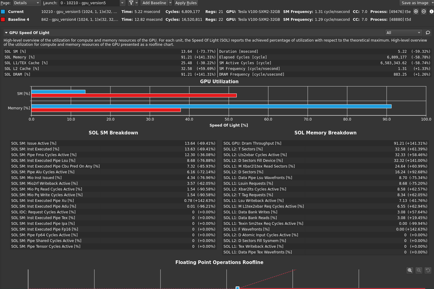
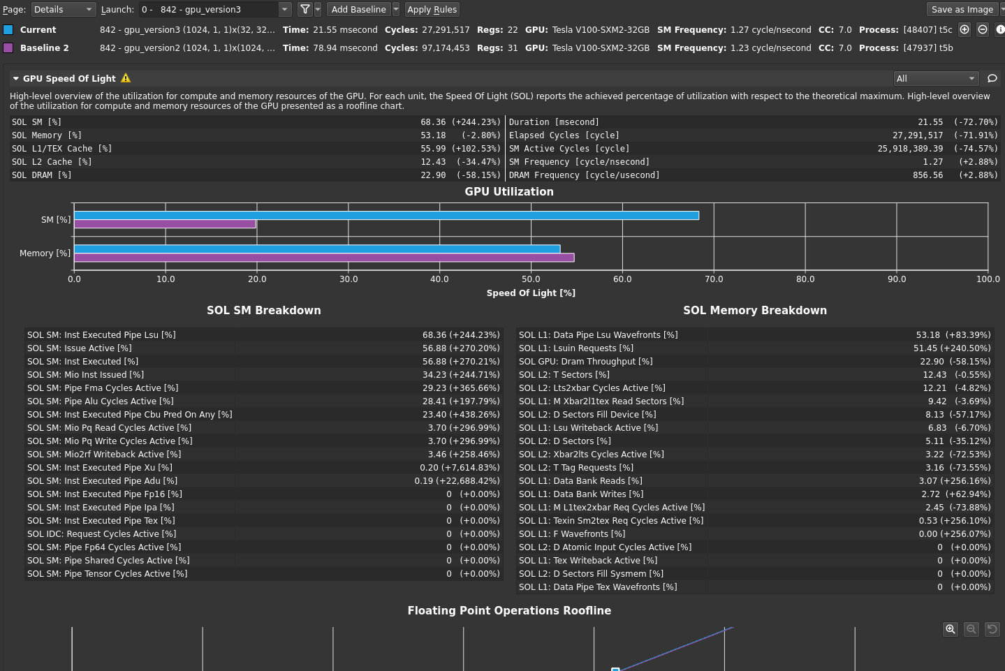
A nice feature of the profiler is the baseline capability. Because you are profiling almost the same kernel, it is interesting to do a comparison in the profiler from your previous results to your current result. To do this, select the previous results tab, choose Add Baseline, and select the latest tab (Figure 1).
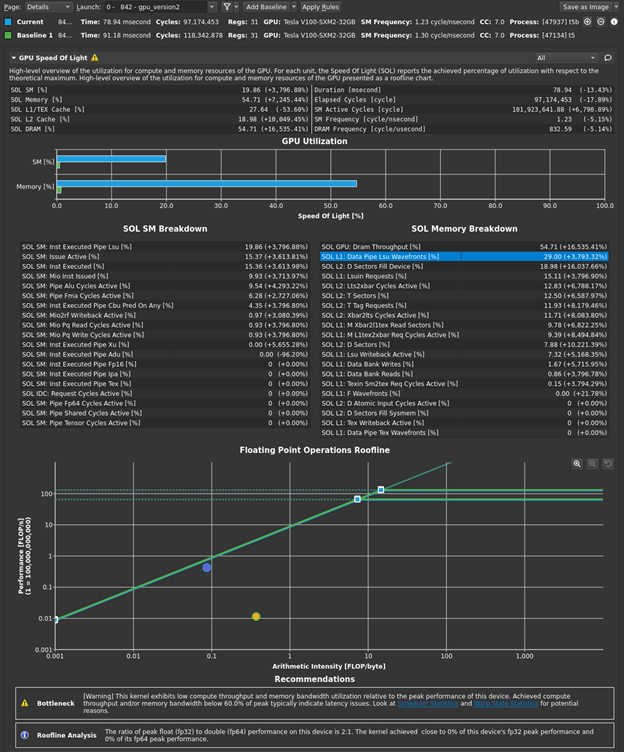
Not all comparisons are meaningful, because the two profiling runs had significantly different N values. Therefore, kernel duration, for example, won’t be directly comparable. However, GPU utilization has improved substantially. The intent here is to let the profiler guide your optimization efforts. Start by inspecting the rules outputs. The bottleneck rule in the SOL section states the following:
[Warning] This kernel exhibits low compute throughput and memory bandwidth utilization relative to the peak performance of this device. Achieved compute throughput and/or memory bandwidth below 60.0% of peak typically indicate latency issues. Look at Scheduler Statistics and Warp State Statistics for potential reasons.
Look at the Scheduler Statistics section (Figure 2).
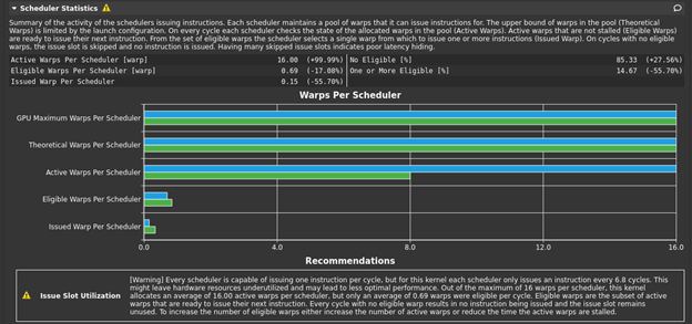
There is another rule in this section, called Issue Slot Utilization, which is reporting as follows:
[Warning] Every scheduler is capable of issuing one instruction per cycle, but for this kernel each scheduler only issues an instruction every 6.8 cycles. This might leave hardware resources underutilized and may lead to less optimal performance. Out of the maximum of 16 warps per scheduler, this kernel allocates an average of 16.00 active warps per scheduler, but only an average of 0.69 warps were eligible per cycle. Eligible warps are the subset of active warps that are ready to issue their next instruction. Every cycle with no eligible warp results in no instruction being issued and the issue slot remains unused. To increase the number of eligible warps either increase the number of active warps or reduce the time the active warps are stalled.
You have the maximum of 16 warps per scheduler but most of the time, the warps are stalled. About 30% of the time, the warps are stalled so extensively that none can be issued by that scheduler in that cycle.
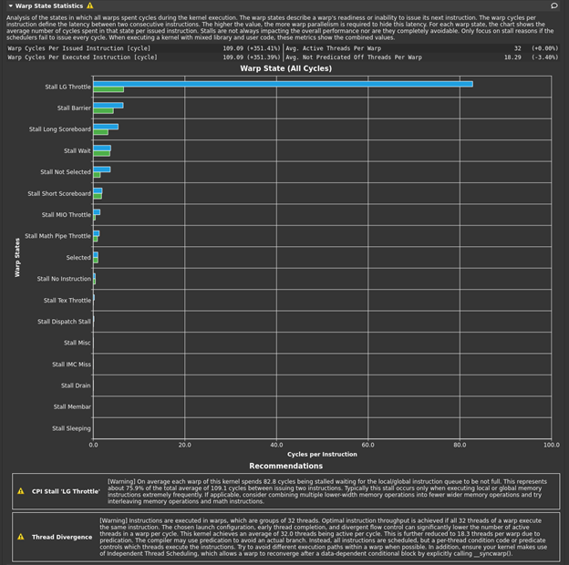
The Warp State Statistics section also has a rule called CPI Stall LG Throttle, as follows:
[Warning] On average each warp of this kernel spends 82.8 cycles being stalled waiting for the local/global instruction queue to be not full. This represents about 75.9% of the total average of 109.1 cycles between issuing two instructions. Typically, this stall occurs only when executing local or global memory instructions extremely frequently. If applicable, consider combining multiple lower-width memory operations into fewer wider memory operations and try interleaving memory operations and math instructions.
You can make a few other observations. The Stall LG Throttle stall reason is listed high, at over 80 cycles. Hover over any bar to get the numerical value. In the Stall LG Throttle legend (on the left side), hover to get a definition of that item, both in terms of the metric calculation used and a text description, “average # of warps resident per issue cycle, waiting for a free entry in the LSU instruction queue”. LSU is Load/Store Unit, one of the functional units in a GPU SM. For more information, see Warp Scheduler States and Metrics Decoder.
Because the directives so far have blended local and global activity together, you can also get a clue about the likely candidate by looking at the Memory Workload Analysis section (Figure 4).
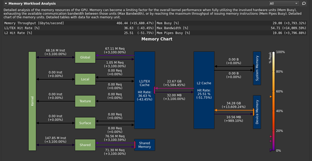
The Memory (hierarchy) Chart shows on the top left arrow that the kernel is issuing instructions and transactions targeting the global memory space, but none are targeting the local memory space. Global is where you want to focus.
Assembling the observations so far, you could conjecture that because the LSU queue is backed up with instructions targeting the global space, but the overall memory utilization is only in the range of ~50% (from the SOL section), perhaps the issue is one of transaction efficiency. For global transactions, transaction efficiency is high when the number of transactions per request is minimized.
At this point, you could profile your kernel again, asking for a global transaction efficiency measurement as you did in the previous post. However, that may only confirm what you already suspect. You would also like the profiler to direct you to the instructions in the code that are giving rise to this global memory or LSU pressure.
At the top of the current profiler results tab, switch the Page: indicator from Details to Source. For more information, see Source Page. In the new page presented, switch View: from Source and SASS to Source. If you don’t see any source code, it may be that you did not include -lineinfo when compiling your code. Fortunately, your kernel is short, so scroll the window vertically to the gpu_version2 kernel source lines. You may want to adjust column widths by dragging the column dividers at the top of this pane.
Can this source view help you to confirm your suspicions about efficiency, and identify lines of code to focus your efforts? Yes. In this view, the profiler is attributing some statistics, metrics, and measurements to specific lines of code. Scroll the window horizontally until you can see both the Memory Ideal L2 Transactions Global and Memory L2 Transactions Global columns. The first column is just a scaled measurement of the number of requests, the ideal number of transactions that is the minimum. The second column is the actual number of transactions that had to be issued to satisfy those requests. The ratio of these, if greater than 1, gives an indicator of inefficiency in global memory access patterns.
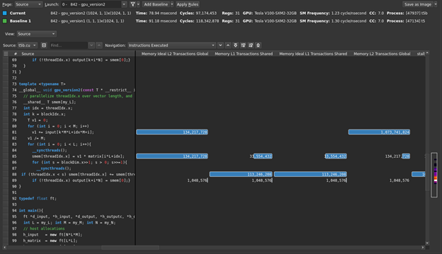
By inspecting the output, you observe that for the following line of code (line 81 in figure 5), the number of ideal transactions would be 134,217,728, whereas the actual number of transactions were much larger, at 1,073,741,824, a ratio of 8:1.
v1 += input[k*M*L+idx*M+i];
This is a good indication from the profiler that this line of code is suffering from a poor or uncoalesced access pattern. On the Details page, confirm your suspicion of uncoalesced access on line 81 by looking at the Source Counters section and its associated rule output at the bottom of the section.
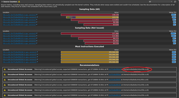
You see that the rule here is also reporting the issue on line 81. By comparison, the following line of code is also doing global accesses, but the corresponding ratio is exactly 1:1:
smem[threadIdx.x] = v1 * matrix[i*L+idx];
Therefore, the access pattern must be fully coalesced. Now, focus your efforts on the first line of code mentioned earlier (line 81), as your next optimization target.
Restructuring
The previous analysis showed uncoalesced access at a particular line of the kernel code. This is because the initial parallelization strategy of one thread per vector element resulted in a thread access pattern for the first phase of the problem that was columnar in memory. Adjacent threads are reading adjacent vector elements, but those adjacent vector elements are not stored in adjacent locations in memory. Your focus now is on the first phase of the algorithm (the vector averaging operation), because the profiler has indicated that the global activity during the second phase (the matrix-vector multiply) is already coalesced. To fix this, your next refactoring effort is more involved.
You must restructure the threads in the first phase, so that adjacent threads are reading adjacent elements in memory. Algorithmically, this is possible because the averaging operation moves horizontally through memory. You therefore want to assign a set of threads that work collectively, instead of just one thread, to process each vector element.
The next logical step up from one thread to a set of threads that can process adjacent elements in memory efficiently would be the warp. Refactor the averaging operation at the threadblock level to be a warp-stride loop moving horizontally, one warp per vector element moving horizontally across vectors, and a block-stride loop moving vertically, so that the threadblock as a whole strides vertically, to cover all the elements in the vector, during the averaging phase. For more information about grid-stride loops, see CUDA Pro Tip: Write Flexible Kernels with Grid-Stride Loops.
Block-stride and warp-stride loops are a variation, operating at the block level or warp level, respectively. Your refactored kernel looks like the following code example:
template
__global__ void gpu_version3(const T * __restrict__ input, T * __restrict__ output, const T * __restrict__ matrix, const int L, const int M, const int N){
  // parallelize threadIdx.x over vector length, and blockIdx.x across k (N)
  // do initial vector reduction via warp-stride loop
  __shared__ T smem[my_L];
  int idx = threadIdx.x;
  int idy = threadIdx.y;
  int id  = idy*warpSize+idx;
  int k = blockIdx.x;
  T v1;
  for (int y = threadIdx.y; y < L; y+=blockDim.y){ // vertical block-stride loop
    v1 = 0;
    for (int x = threadIdx.x; x < M; x+=warpSize)  // horizontal warp-stride loop
      v1 += input[k*M*L+y*M+x];
    for (int offset = warpSize>>1; offset > 0; offset >>= 1) // warp-shuffle reduction
       v1 += __shfl_down_sync(0xFFFFFFFF, v1, offset);
    if (!threadIdx.x) smem[y] = v1/M;}
  __syncthreads();
  v1 = smem[id];
  for (int i = 0; i < L; i++){                     // matrix-vector multiply
    __syncthreads();
    smem[id] = v1 * matrix[i*L+id];
    for (int s = (blockDim.x*blockDim.y)>>1; s > 0; s>>=1){
      __syncthreads();
      if (id < s) smem[id] += smem[id+s];}
    if (!id) output[k+i*N] = smem[0];}
}
You also need to update your kernel launch:
  dim3 block(32,32);
  gpu_version3<<<N, block>>>(d_input, d_output, d_matrix, L, M, N);
If you recompile and run this code, you observe another performance improvement in the kernel:
CPU execution time: 0.539879s
Kernel execution time: 0.021637s
|
|
baseline |
Step 1 |
Step 2 |
|
Kernel duration |
2.92s |
0.0789s |
0.0216s |
To continue the ADO process, return to the profiler. Choose Disconnect, Connect, Launch, and then Run to Next Kernel. After about 10 seconds, you are presented with a new report in a new tab. At this point, you may wish to switch back to the first tab, choose Clear Baselines, move to the previous tab, and choose Add Baseline. Move to the current tab and report. Figure 7 shows the results.

The bottleneck rule states:
[Warning] Compute is more heavily utilized than Memory: Look at the Compute Workload Analysis report section to see what the compute pipelines are spending their time doing. Also, consider whether any computation is redundant and could be reduced or moved to look-up tables.
You’re being directed to the Compute Workload Analysis report section (Figure 8) to determine which pipe is the most heavily utilized.
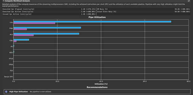
This section doesn’t have any rule warnings, but you see that the LSU pipe is the most heavily utilized. This again suggests pressure associated with memory transactions. Can you determine which memory transactions might be the biggest contributor to this? Look at the next section, Memory Workload Analysis (Figure 9).
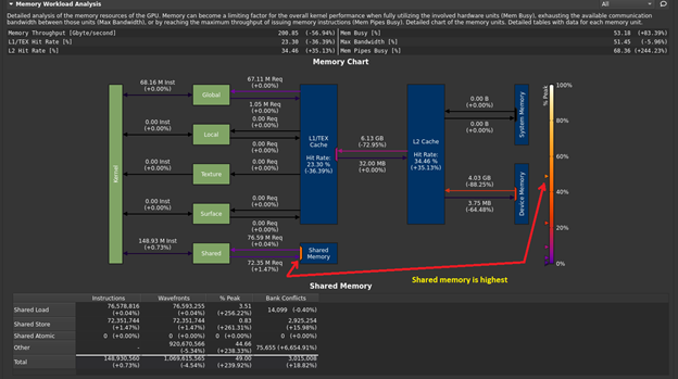
I’ve truncated the bottom portion of the Memory Workload Analysis screen. However, you can study the Memory Chart to see that the shared-memory usage is the highest reported usage, at 49% of peak. If you are going to focus on LSU cycle pressure, the attention shifts to shared-memory activity. As a result of the sweep-style reduction construction considered across the threadblock, there are many iterations of the sweep reduction loop that have one or more entire warps that do not participate. They are predicated off, completely across the warp. These non-participating warps still contribute to shared-memory pressure, and this is reflected in the Other category in the screenshot.
Figure 10 shows the source display, focusing on the kernel code.
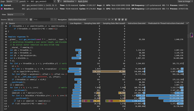
The profiler has indicated, based on warp-state sampling, that the following line accounts for many shared-memory-related warp stalls (line 114 in figure 10):
if (id < s) smem[id] += smem[id+s];}
This line of code is doing two loads and one store from/to shared memory, as part of your sweep reduction. Coupled with the previous analysis, this becomes the focus for your next optimization.
Summary
In this post, you continued the ADO process started in part 1, by applying what you learned in this post to refactor the code, and profile again to discover next steps. In part 3, you finish your analysis and optimization. You also perform some measurements to give you confidence that you have reached a reasonable stopping point.
The analysis work in this post was performed on a machine with the following characteristics: Ubuntu 18.04.3, CUDA 11.1, GPU Driver version 455.23.05, GCC version 7.5.0, V100-SXM2-32 GB GPU, Intel® Xeon® Gold 6130 CPU @ 2.10GHz. The code examples presented in this post are for instructional purposes only. They are not guaranteed to be defect-free or suitable for any particular purpose.
For more information, see the following resources:
- Hands-on optimization tutorial for NVIDIA Nsight tools
- GPU Performance Analysis video (part 8 of a 9-part CUDA Training Series that NVIDIA presented for OLCF and NERSC)
- Accelerating HPC Applications with NVIDIA Nsight Compute Roofline Analysis.
- Roofline and NVIDIA Ampere GPU Architecture Analysis video
Acknowledgements
The author would like to thank the following individuals for their contributions: Sagar Agrawal, Rajan Arora, Ronny Brendel, Max Katz, Felix Schmitt, Greg Smith, and Magnus Strengert.