This tutorial is the fifth installment of introductions to the RAPIDS ecosystem. The series explores and discusses various aspects of RAPIDS that allow its users solve ETL (Extract, Transform, Load) problems, build ML (Machine Learning) and DL (Deep Learning) models, explore expansive graphs, process geospatial, signal, and system log data, or use SQL language via BlazingSQL to process data.
The emergence of social networks such as LinkedIn, Twitter, or Facebook brought extensive and complex graphs into existence and everyday use, graphs with billions of nodes and hundreds of billions if not trillions of edges. Processing graphs of this scale that can scale to handle large objects and able to process data fast.
RAPIDS cuGraph was introduced shortly after RAPIDS’ initial release. Each release since then brought new functionality, either in the form of new algorithms or enabling existing algorithms to scale to multi-node, multi-GPU clusters.

The previous posts in the series showcased other areas:
- In the first post, python pandas tutorial, we introduced cuDF, the RAPIDS DataFrame framework for processing large amounts of data on an NVIDIA GPU.
- The second post compared similarities between cuDF DataFrame and pandas DataFrame.
- In the third post, data processing with Dask, we introduced a Python distributed framework to run distributed workloads on GPUs.
- In the fourth post, the functionality of cuML, we introduced the Machine Learning library of RAPIDS.
In this tutorial, we introduce and showcase the most common functionality of RAPIDS cuGraph. As with cuDF or cuML, to get familiar with cuGraph we have provided a cuGraph cheatsheet.
The rise of Skywalk… I mean – graphs! graphs!
Graphs were first formally introduced in the early 18th century by Euler to solve one of the famous-at-the-time problems: the Königsberg Bridge Problem. The problem is still famous today, studied in computer science classes and asked during many software engineer interviews. As it was stated, the problem asked a simple question: is there a way to cross each of the bridges of Königsberg (today’s Kaliningrad) exactly once while on a stroll? Euler’s solution used graphs to answer this question once and for all: it is not possible to cross each of the bridges while walking through the city!
Graphs and graph theory nowadays can be found almost everywhere. Airlines and delivery services use graph theory to optimize their schedules given their fleet’s composition and size or assign vehicles and cargo for each route. Internet and local networks can be viewed as graphs; social network companies use graph theory to find influencers and cliques (communities or groups) of friends. Government investigative bodies study graphs to identify potential terrorist threats or cells.
Graphs also take a prominent place in data science. If you have ever trained a neural network or used a data distributed data processing framework that implements a lazy execution paradigm (like Dask or Spark), you might have heard the term DAG or a Directed Acyclic Graph. A deep learning model can be represented as DAG, where a neuron in one layer is connected to another neuron in the next layer via weight (an edge of the graph), while a neuron in this graph constitutes a node (or vertex). Similarly, as you add more transformations to your Dask DataFrame, another set of nodes (tasks) is added to the execution graph, where edges indicate the flow of results between tasks.
Graphs are everywhere!
Ever-growing data and networks
In practice, graphs consisting of only 7 nodes (like the Königsberg graph) are rarely found. More often, we deal with graphs of thousands, millions, and billions of nodes and an associated number of edges that practically always is a multiple of the count of nodes.
When the Internet’s predecessor, the ARPANET, was in its nascent stage, the graph of that network consisted of only two nodes and a single edge. Today, computers and TVs, cameras, phones, and IoT devices are getting connected in droves every day. We have a massive network of billions of devices, and their communication graph contains trillions (if not more) edges.
Nearly 2.6bn Facebook users log in at least once per month, and around 1.7bn of them do so daily. Let’s think about this graph for a second: even if each of the daily Facebook users checked only one Facebook page, we would have a graph of 1.7bn + 1 (the page) edges. It is hard to believe that a user would only check one page so let’s complicate things further: assume that every Facebook user sees the same page with 10 posts on it. We now have a graph with 17bn edges (and an edge’s attribute could be viewed as – a user foo has seen post-bar). The process doesn’t stop here: as you might envisage the graph will grow with edges for ‘likes’ or ‘clicks’ as well.
The numbers are mind-boggling, and it’s only one site. When you think that the Google index contains around 50 billion pages, we are now encroaching on a realm of astronomically large graphs. Many companies need tools to process these graphs and extract insights or build models. After all, their business models depend on it. NVIDIA cuGraph is a leap towards making graph analytics and processing large graphs possible in near-real-time (or minutes rather than days).
Create a graph using cuGraph
In cuGraph, you can create a graph by either passing an adjacency list or an edge list.
The adjacency list is a Compressed Sparse Row representation of the graph’s adjacency matrix. The adjacency matrix is a V-by-V (where V is the number of nodes in the graph) matrix where a value at point (x,y) indicates an edge between node x and y.The edge list is simply a list of the pairs (x,y) with optionally some associated weight for each edge.
import cugraph
from scipy.sparse import coo_matrix

values = [1,1,1,1,1]
sources = [0,0,0,1,2]
destinations = [1,2,3,2,3]

adj_list = coo_matrix((values, (sources, destinations))).tocsr()

g = cugraph.Graph()
g.from_cudf_adjlist(cudf.Series(adj_list.indptr), cudf.Series(adj_list.indices))
In cuGraph, the edge list is commonly a DataFrame where each row indicates an edge. At minimum, the DataFrame needs to have two columns: source node and destination node; in order to create a weighted graph you can include a third column as an edge attribute.
edges = cudf.DataFrame([
(0, 1, 1)
, (0, 2, 1)
, (0, 3, 1)
, (1, 2, 1)
, (2, 3, 1)
], columns=['src', 'dst', 'weight'])

g = cugraph.Graph()
g.from_cudf_edgelist(
edges
, source='src'
, destination='dst'
, edge_attr='weight'
, renumber=False
)
Finding influencers
One of the most fundamental questions you can ask a graph is “who are the influencers?” That is, in the case of social networks, how do I find people who I can reach out to, connect with, and tap into their network to market my product or service? cuGraph can calculate multiple measures of centrality for each node or edge. The betweenness_centrality metric, in terms of a social network, calculates how many times a person would be asked to convey an introduction message to one of their connections.
cugraph.betweenness_centrality(g, k=20, normalized=True, weight=None)The Katz Centrality metric, on the other hand, measures how many different ways one person can reach another and how many times each node occurs in such walks.
cugraph.katz_centrality(g, alpha=0.05, max_iter=200, tol=1e-07)
Finding communities
Finding communities, or cliques, in a graph is another important aspect of mining information from a graph. For example, finding bad guys that are trying to steal the data in a network of a bank might involve analyzing the normal communications pattern between a community of machines and then detect change in these patterns. A new node added or an increased amount of packets transmitted might give away an attempt.
cuGraph implements many community finding algorithms, starting with the most frequently used Louvain, an algorithm that optimizes the modularity metric; the modularity measures the relative density of edges inside communities with respect to the edges outside the community.
parts, modularity_score = cugraph.louvain(g, max_iter=10)
Leiden algorithm is an extension of the Louvain algorithm and it guarantees that the communities are well-connected.
parts, modularity_score = cugraph.leiden(g, max_iter=10)
To further explore all the community finding algorithms, check the cuGraph cheatsheet.
Exploring the graph structure, or how to not get lost
When you use a GPS to guide you to your destination, the algorithm inside the unit effectively solves a graph algorithm to find the shortest path between two nodes. Road intersections, individual addresses, or landmarks can be viewed as nodes of an undirected graph; roads themselves form the edges. The shortest path algorithm explores the graph and returns a sequence of hops for you to follow (yes, the familiar turn right in 300ft messages) in such a way that it minimizes the travel distance. You can, of course, change the edge attribute to time and instead of prioritizing the shortest distance, you will be optimizing for a minimal travel time. Thanks, graphs! Oh, and here how simple it is to find all shortest paths from node 0 to all other nodes using cuGraph.
cugraph.shortest_path(g, 0)
Explore the capabilities of cuGraph by downloading the cuGraph cheatsheet!
