Over the past couple of years, NVIDIA and NASA have been working closely on accelerating data science workflows using RAPIDS and integrating these GPU-accelerated libraries with scientific use cases. In this blog, we’ll share some of the results from an atmospheric science use case, and code snippets to port existing CPU workflows to RAPIDS on NVIDIA GPUs.
Accelerated Simulation of Air Pollution from Christoph Keller
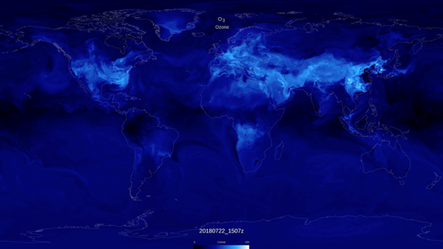
One example science use case from NASA Goddard simulates chemical compositions of the atmosphere to monitor, forecast, and better understand the impact of air pollution on the environment, vegetation, and human health. Christoph Keller, a research scientist at the NASA Global Modeling and Assimilation Office, is exploring alternative approaches based on machine learning models to simulate the chemical transformation of air pollution in the atmosphere. Doing such calculations with a numerical model is computationally expensive, which limits the use of comprehensive air quality models for real-time applications such as air quality forecasting. For instance, the NASA GEOS composition forecast model GEOS-CF, which simulates the distribution of 250 chemical species in the Earth atmosphere in near real-time, needs to be run on more than 3000 CPUs and more than 50% of the required compute cost is related to the simulation of chemical interactions between these species.
We were able to accelerate the simulation of atmospheric chemistry in the NASA GEOS Model with GEOS-Chem chemistry more than 10-fold by replacing the default numerical chemical solver in the model with XGBoost emulators. To train these gradients boosted decision tree models, we produced a dataset using hourly output from the original GEOS model with GEOS-Chem chemistry. The input dataset contains 126 key physical and chemical parameters such as air pollution concentrations, temperature, humidity, and sun intensity. Based on these inputs, the XGBoost model is trained to predict the chemical formation (or destruction) of an air pollutant under the given atmospheric conditions. Separate emulators are trained for individual chemicals.
To make sure that the emulators are accurate for the wide range of atmospheric conditions found in the real world, the training data needs to capture all geographic locations and annual seasons. This results in very large training datasets – quickly spanning 100s of millions of data points, making it slow to train. Using RAPIDS Dask-cuDF (GPU-accelerated dataframes) and training XGBoost on an NVIDIA DGX-1 with 8 V100 GPUs, we are able to achieve 50x overall speedup compared to Dual 20-Core Intel Xeon E5-2698 CPUs on the same node.
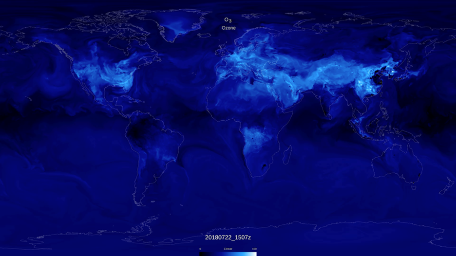
An example of this is given in the gc-xgb repo sample code, showcasing the creation of an emulator for the chemical compound ozone (O3), a key air pollutant and climate gas. For demonstration purposes, a comparatively small training data set spanning 466,830 samples is used. Each sample contains up to 126 non-zero features, and the full size of the training data contains 58,038,743 entries. In the provided example, the training data – along with the corresponding labels – is loaded from a pre-generated txt file in svmlight / libsvm format, available in the GMAO code repo:
Loading the training data from a pre-generated text file, as shown in the example here, sidesteps the data preparation process whereby the 4-dimensional model data (latitude x longitude x altitude x time) as generated by the GEOS model (in netCDF format) are being read, subsampled and flattened.
The loaded training data can directly be used to train an XGBoost model:
Setting the tree_method to ‘gpu_hist’ instead of ‘hist’ performs the training on GPUs instead of CPUs, highlighting a significant speed-up in training time even for the comparatively small sample training data used in this example. This difference is exacerbated on the much larger data sets needed for developing emulators suitable for actual use in the GEOS model. Since our application requires training of dozens of ML emulators – ideally on a recurring basis as new model data is produced – the much shorter training time on RAPIDS is critical and ensures a short enough model development cycle.
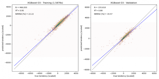
As shown in the figure below, the chemical tendencies of ozone (i.e., the change in ozone concentration due to atmospheric chemistry) predicted by the gradient boosted decision tree model shows good agreement with the true chemical tendencies simulated by the numerical model. Given the relatively small training sample size (466,830 samples), the here trained model shows some signs of overfitting, with the correlation coefficient R2 dropping from 0.95 for the training data to 0.88 in the validation data, and the normalized root means square error (NRMSE) increasing from 22% to 35%. This indicates that larger training samples are needed to ensure that the training dataset captures all chemical environments.
In order to deploy the XGBoost emulator in the GEOS model as a replacement to the GEOS-Chem chemical solver, the XGBoost algorithm needs to be called from within the GEOS modeling system, which is written in Fortran. To do so, the trained XGBoost model is saved to disk so that it can then be read (and evoked) from a Fortran model by leveraging XGBoost’s C API (The XGBoost interface for Fortran can be found in the fortran2xgb GitHub repo.
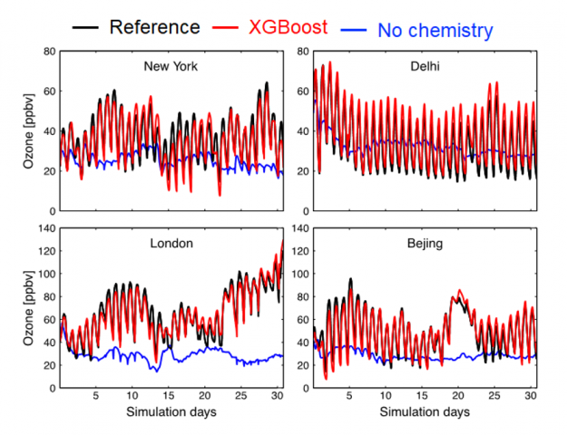
As shown in the figure below, running the GEOS model with atmospheric chemistry emulated by XGBoost produces surface ozone concentrations that are similar to the numerical solution (red vs. black line). The blue line shows a simulation using a model with no chemistry, highlighting the critical role of atmospheric chemistry for surface ozone.
GEOS model simulations using XGBoost emulators instead of the GEOS-Chem chemical solver have the potential to be 20-50% faster than the reference simulation, depending on the model configuration (such as horizontal and temporal resolution). By offering a much faster calculation of atmospheric chemistry, these ML emulators open the door for a range of new applications, such as probabilistic air quality forecasts or a better combination of atmospheric observations and model simulations. Further improvements to the ML emulators can be achieved through mass balance considerations and by accounting for error correlations, tasks that Christoph and colleagues are currently working on.
In the next blog, we’ll talk about another application leveraging XGBoost and RAPIDS for live monitoring of air quality across the globe during the COVID-19 pandemic.
References:
Keller, C. A., Clune, T. L., Thompson, M. A., Stroud, M. A., Evans, M. J., and Ronaghi, Z.: Accelerated Simulation of Air Pollution Using NVIDIA RAPIDS, GPU Technology Conference, https://ntrs.nasa.gov/archive/nasa/casi.ntrs.nasa.gov/20190033152.pdf, 2019.
Keller, C. A. and Evans, M. J.: Application of random forest regression to the calculation of gas-phase chemistry within the GEOS-Chem chemistry model v10, Geosci. Model Dev., 12, 1209–1225, https://doi.org/10.5194/gmd-12-1209-2019, 2019.