
朴素贝叶斯( NB )是一种简单但功能强大的概率分类技术,具有良好的并行性,可以扩展到大规模数据集。
如果您一直从事数据科学中的文本处理任务,您就会知道 机器学习 模型可能需要很长时间来训练。在这些模型上使用 GPU 加速计算通常可以显著提高时间性能, NB 分类器也不例外。
通过使用 CUDA 加速操作,根据使用的 NB 模型,我们实现了从 5 到 20 倍的性能提升。对稀疏数据的智能利用使其中一个模型的速度提高了 120 倍。
在本文中,我们介绍了 RAPIDS cuML 中 NB 实现的最新升级,并将其与 Scikit-learn 在 CPU 上的实现进行了比较。我们提供基准测试来演示性能优势,并通过算法的每个支持变量的简单示例来帮助您确定哪个最适合您的用例。
什么是朴素贝叶斯?
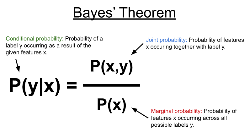
NB 使用 Bayes’ theorem (图 1 )对如下所示的条件概率分布进行建模,以预测给定一些输入特征( x )的标签或类别( y )。在其最简单的形式中,贝叶斯定理使用特征和可能标签之间的联合概率以及特征在所有可能标签上出现的边际概率来计算条件概率。
NB 算法在文本分类用例中表现良好。它们通常用于过滤垃圾邮件等任务;预测推特、网页、博客帖子、用户评分和论坛帖子的类别和情感;或对文档和网页进行排名。
NB 算法通过使每个特征(例如,输入向量 x 中的每列)在统计上独立于所有其他特征来简化条件概率分布 naive assumption 。这使得该算法很棒,因为这种天真的假设提高了算法的并行化能力。此外,计算特征和类标签之间简单共生概率的一般方法使模型能够进行增量训练,支持不适合内存的数据集。
NB 有几种变体,它们对各种类别标签的联合分布或共同出现的特征进行了某些假设。
朴素贝叶斯假设
为了预测未知输入特征集的类别,关于联合分布的不同假设使算法具有几种不同的变体,该算法通过学习不同概率分布的参数来建模特征分布。
表 1 模拟了一个简单的文档/术语矩阵,该矩阵可以来自文本文档集合。列中的术语代表一个词汇表。一个简单的词汇表可能会将一个文档分解为一组在所有文档中出现的唯一单词。
| I | love | dogs | hate | and | knitting | is | my | hobby | session | |
| Doc 1 | 1 | 1 | 1 | |||||||
| Doc 2 | 1 | 1 | 1 | 1 | 1 | |||||
| Doc 3 | 1 | 1 | 1 | 2 | 1 | 1 |
表 1 . 包含沿行文档和沿列出现在每个文档中的词汇的文档/术语矩阵
在表 1 中,每个元素可以是一个计数,如此处所示, 0 或 1 表示特征的存在,或其他一些值,如在整个文档集上出现的每个项的比率、扩散或离散度。
在实践中,滑动窗口通常在整个文档或术语上运行,将它们进一步划分为小块的单词序列,称为 n-grams 。对于下图的第一个文档, 2-gram (或 bigram )将是“ I love ”和“ love dogs ”。这类数据集中的词汇通常会显著增大并变得稀疏。预处理步骤通常在词汇表上执行,以过滤噪声,例如,通过删除大多数文档中出现的常见术语。
将文档转换为文档项矩阵的过程称为矢量化。有一些工具可以加速这个过程,例如 CountVectorizer cuML 中的 CountVectorizer 、 TdfidfVectorizer 或 RAPIDS 估计器对象。
多项式和伯努利分布
表 1 表示一组文档,这些文档已矢量化为术语计数,结果矩阵中的每个元素表示特定单词在其相应文档中出现的次数。这种简单的表示方法可以有效地用于分类任务。
由于特征代表频率分布,多项式朴素贝叶斯变体可以有效地将特征及其相关类别的联合分布建模为多项式分布。
可以通过合并色散度量来增强每个项的频率分布,例如项频率逆文档频率( TF-IDF ),它考虑了每个项中出现的文档数量。这可以通过对出现在较少文档中的术语赋予更多权重来显著提高性能,从而提高其识别能力。
虽然多项式分布在直接与项频率一起使用时效果很好,但它也被证明在分数值上有很好的性能,如 TF-IDF 值。多项式朴素贝叶斯变体涵盖了大量用例,因此往往是使用最广泛的。类似的变体是伯努利朴素贝叶斯,它模拟每个项的简单出现,而不是它们的频率,从而得到 0 和 1 的矩阵(伯努利分布)。
不等阶级分布
在现实世界中,经常会发现不平衡的数据集。例如,您可能有有限的垃圾邮件和恶意活动的数据样本,但有丰富的正常和良性样本。
补码朴素贝叶斯变体通过在训练期间为每个类使用联合分布的补码,例如,在所有其他类的样本中出现特征的次数,有助于减少不平等类分布的影响。
分类分布
你也可以为你的每一个特征创建存储箱,可能通过将一些频率量化到多个存储桶中,使得 0-5 的频率进入存储桶 0 , 6-10 的频率进入存储桶 1 ,等等。
另一种选择是将几个术语合并到一个功能中,可能是为“动物”和“假日”创建桶,其中“动物”可能有三个桶,零个用于猫科动物,一个用于犬科动物,两个用于啮齿动物。“假日”可能有两个桶,零用于个人假日,如生日或结婚纪念日,一个用于联邦假日。
分类朴素贝叶斯 变体假设特征遵循分类分布。朴素假设在这种情况下效果很好,因为它允许每个特征都有一组不同的类别,并且它使用(您猜对了)分类分布对联合分布进行建模。
连续分布
最后,当特征是连续的时,高斯朴素贝叶斯 变体非常有效,可以假设每个类别中的特征分布可以用高斯分布建模,即用简单的均值和方差。
虽然这种变体在 TF-IDF 归一化后可能在某些数据集上表现出良好的性能,但它在一般机器学习数据集上也很有用。
| Algorithm | Multinomial | Bernoulli | Complement | Categorical | Gaussian |
| Type of input | Frequencies, Counts | Boolean occurrence | Counts | Categorical | Continuous |
| Advantage | Support count data | Support binary data | Reduce impact of imbalance data | Support categorical data | Support general continuous data |
表 2.不同 NB 算法的比较 s
真实世界的端到端示例
如表 2 所示,为了证明每种算法变体的优点,我们逐步浏览了每种算法变体的示例笔记本。有关包含所有示例的全面端到端笔记本,请参阅 news_aggregator_a100.ipynb 。
我们使用新闻聚合器数据集来演示 NB 变体的性能。该数据集可从 Kaggle 公开获取,由来自多个新闻来源的 422K 条新闻标题组成。每个标题都标有四个可能的标签之一:商业、科技、娱乐和健康。使用 cuDF RAPIDS 将数据直接加载到 GPU 上,并继续执行针对每个 NB 变体的预处理步骤。
高斯朴素贝叶斯
从高斯朴素贝叶斯 , 开始,我们运行 TD-IDF 矢量器将文本数据转换为可用于训练的实值向量。
通过指定ngram_range=(1,3),我们表示我们将学习单字以及 2-3-gram 。这显著增加了要学习的术语或功能的数量,从 15K 个单词增加到 180 万个组合。由于大多数术语不会出现在大多数标题中,因此生成的矩阵稀疏,许多值等于零。 cuML 支持特殊结构来表示这样的数据。
NB 分类器的另一个优点是,可以使用partial_fit方法对Estimator对象进行增量训练。这种技术适用于可能无法一次性放入内存或必须分布在多个 GPU 中的大规模数据集。
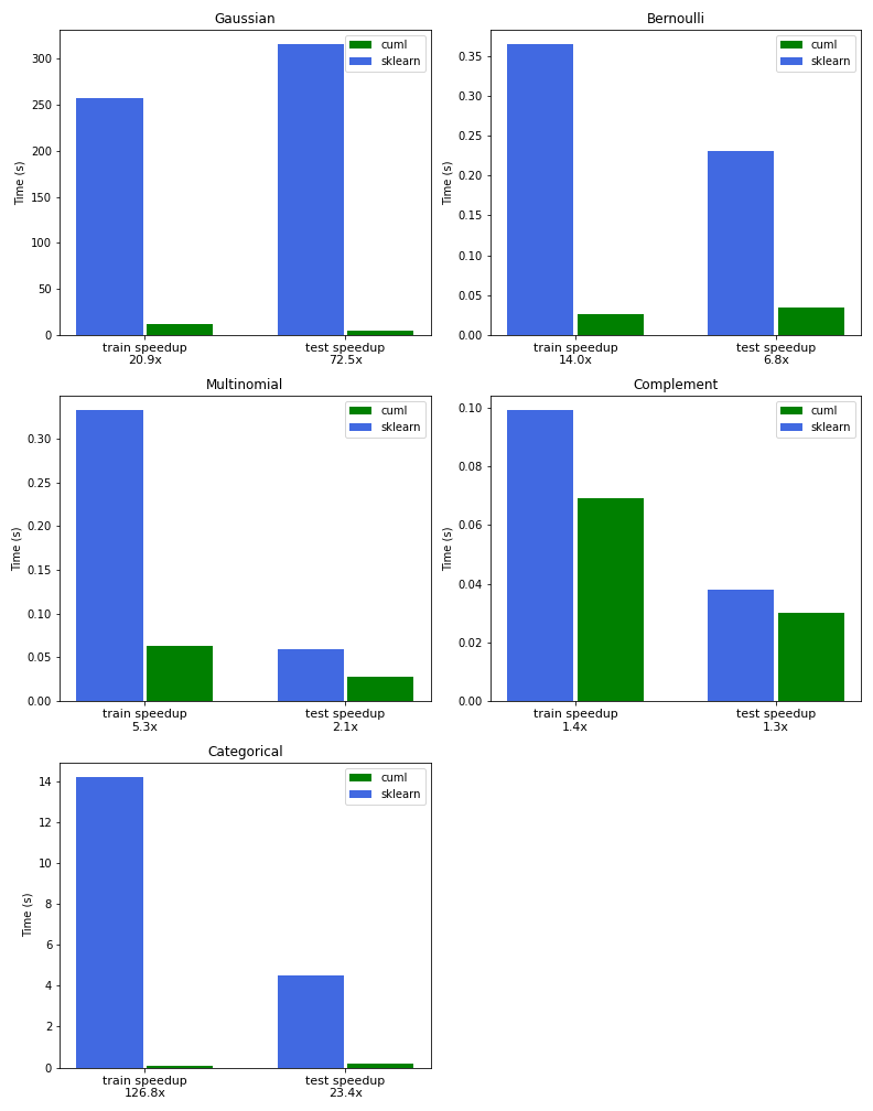
我们的第一个示例演示了使用高斯朴素贝叶斯的增量训练,方法是在使用 TF-IDF 预处理为连续特征后,将数据分割成多个块。高斯朴素贝叶斯的 cuML 版本在训练方面比 Scikit 学习快 21 倍,在推理方面快 72 倍。
伯努利朴素贝叶斯
下一个示例演示了伯努利朴素贝叶斯,无需增量训练,使用表示每个项存在或不存在的二进制特征。CountVectorizer对象可以通过设置binary=True来实现这一点。在本例中,我们发现比 Scikit learn 快 14 倍。
多项式朴素贝叶斯
多项式朴素贝叶斯是最通用和最广泛使用的变体,如以下示例所示。我们使用 TF-IDF 矢量器而不是CountVectorizer来实现比 Scikit learn 快 5 倍的速度。
补码朴素贝叶斯
我们使用CountVectorizer证明了补码朴素贝叶斯的威力,并表明在我们的不平衡数据集上,它比伯努利和多项式 NB 变体产生了更好的分类分数。
范畴朴素贝叶斯
最后但绝对不是最不重要的是一个分类朴素贝叶斯的例子,我们使用 k-means 和之前在另一个 NB 变体上训练的模型对其进行矢量化,以根据相似项对结果类的贡献将其分组到相同的类别中。
我们发现,与 Scikit 相比,使用 315K 条新闻标题训练模型的速度提高了 126 倍,使用 23 倍的速度进行推理和计算模型的准确性。
基准
图 2 中的图表比较了 RAPIDS cuML 和 Scikit learn 之间的 NB 训练和推理的性能,以及本文中概述的所有变体。
基准测试是在a2-highgpu-8g谷歌云平台( GCP )实例上执行的,该实例配备了 NVIDIA Tesla A100 GPU 和 96 Intel Cascade Lake v CPU ,频率为 2.2Ghz 。
GPU 加速朴素贝叶斯
我们能够使用 CuPy 在 Python 中实现所有 NB 变体,这是一种 GPU 加速,几乎可以替代 NumPy 和 SciPy 。 CuPy 还提供了用 Python 编写自定义 CUDA 内核的功能。当 Python 应用程序运行时,它使用 NVRTC 的即时( JIT )编译功能在 GPU 上编译和执行它们。
所有 NB 变体的核心是两个使用 CuPy 的 JIT 编写的简单原语,用于汇总和计算每个类的特征。
当单个文档项矩阵过大而无法在单个 GPU 上处理时, Dask 库可以利用增量训练功能将处理扩展到多个 GPU 和多个节点。目前,多项式变量可以在 cuML 中与 Dask 一起分布。
结论
NB 算法应该在每个数据科学家的工具包中。使用 RAPIDS cuML ,您可以在 GPU 上加速 NB 的实现,而无需大幅更改代码。这些强大而基本的算法,再加上 cuML 的加速,提供了您必须在超大或稀疏数据集上执行分类的一切。
如果你认为 RAPIDS cuML 可以帮助加速你的数据科学和机器学习工作流程,或者已经在这样做了,那么请留下评论,因为我们很乐意听到。
一如既往,请访问 rapidsai GitHub repo ,让我们知道我们可以如何帮助您。你也可以在推特上 @rapidsai 关注我们。
如果您是 RAPIDS 新手,请务必查看 Getting Started 资源以快速启动和运行。