Software profiling is key for achieving the best performance on a system and that’s true for the data science and machine learning applications as well. In the era of GPU-accelerated deep learning, when profiling deep neural networks, it is important to understand CPU, GPU, and even memory bottlenecks, which could cause slowdowns in training or inference.
In this post, we explore many ways of profiling, from the basics to more advanced techniques. We also provide some tips and tricks to optimize deep learning models based upon the profiling results.
Before diving deep into profiling, here are some logistics. We used a ResNet50-based image classification model on different frameworks, such as TensorFlow and PyTorch. When we profiled the ResNet50 model using TensorFlow and PyTorch, we used the most recent and performant NVIDIA A100 GPU on a NVIDIA DGX A100 system. This GPU has 40 GB of memory and has support for multiple data types, including the new data type TensorFloat-32 (TF32). We employed a variety of tools for profiling to show you the alternatives.
nvidia-smi
The first go-to tool for working with GPUs is the nvidia-smi Linux command. This command brings up useful statistics about the GPU, such as memory usage, power consumption, and processes running on GPU. The goal is to see if the GPU is well-utilized or underutilized when running your model.
First, check how much GPU memory you are utilizing. You usually want to see your models using most of the available GPU memory—especially while training a deep learning model—as it is an indicator of a well-utilized GPU. Power consumption is another strong indicator of GPU utilization. Typically, the more CUDA or Tensor Cores that are fired up, the more GPU power is consumed.
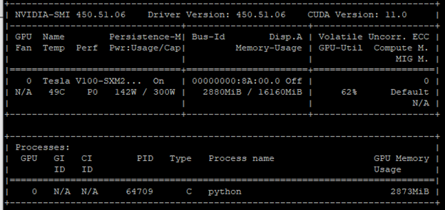
Figure 1 shows an underutilized GPU. This conclusion was formed from two metrics:
- Power consumption: 142 W / 300 W
- Memory usage: 2880 MB / 16160 MB
The GPU-utilization (GPU-Util) column confirms this conclusion with a rate of 62%. One remedy is to increase the batch size. More cores are fired to process a larger batch size. As a result, you get more out of the GPU.
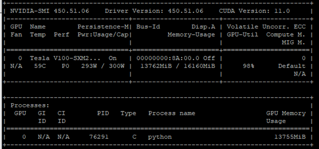
Increase the batch size and make the same Python program call. Figure 2 shows a GPU utilization of 98%. You can confirm this finding when you check the power consumption and memory usage. They are close to their limits.
You did your first optimization. Using a larger batch size (that is, a batch size that occupies almost all the GPU memory) is the most common optimization technique in the deep learning world to improve GPU utilization.
Power consumption and memory usage are not the only metrics that nvidia-smi reveals. You can also try nvidia-smi dmon, which prints out more statistics about the GPU in a scrolling manner (Figure 3).
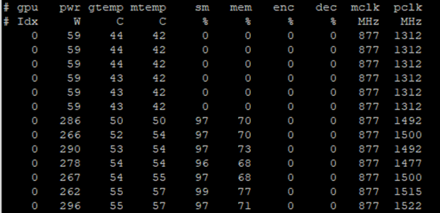
nvidia-smi dmon printing more statistics about the GPU utilization.Each GPU has several streaming multiprocessors (SMs), which run the CUDA kernels. Using many SMs is a signal of a well-utilized GPU. Figure 3 shows that SM utilization starts around 0% when the call starts and then climbs up to the upper 90s when the actual training starts. In addition to the SM utilization, nvidia-smi dmon prints the following statistics:
- Power consumption (pwr)
- GPU temperature (gtemp)
- Memory temperature (mtemp)
- Memory utilization (mem)
- Encoder utilization (enc)
- Decoder utilization (dec)
- Memory clock rate (mclk)
- Processor clock rate (pclk)
So far, you have focused on using only one GPU. In the case of multiple GPUs, nvidia-smi and nvidia-smi dmon show metrics separately for each GPU. Another tool that you can leverage when you have multiple GPUs is nvidia-topo -m. This call displays the topology of the GPU devices and how they are connected to each other.
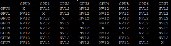
Figure 4 shows the topology configuration on a DGX A100 system with 8x A100 GPUs connected with NVLink. When choosing specific GPUs to run your workload, you may want to pick the NVLink-connected GPUs as they would have higher bandwidth, especially on DGX-1 systems.
So far, we have shown you how to analyze GPU utilization using the nvidia-smi tool. These metrics are indicators of an underutilized or a well-utilized GPU. In your modeling, you should always aim at fully harnessing GPUs to better leverage the accelerated computing.
TensorFlow and DLProf
GPU utilization is a great starting point for profiling and optimization. You can do more analysis of modeling in detail by employing tools like DLProf and PyProf. You can also take advantage of user interfaces to visually inspect your code. Deep Learning Profiler (DLProf) provides support for TensorBoard so that you can visually inspect your models.
The following code example trains a ResNet50 model with TensorFlow 1.15. It also hooks up DLProf parameters to get the profiling running while training your model.
dlprof --nsys_opts="--sample=cpu --trace 'nvtx,cuda,osrt,cudnn'" \
--profile_name=/ecan/tf_a100_profiling --nsys_base_name=resnet50_tf_fp32_b408 \
--output_path=/ecan/tf_a100_profiling --tb_dir=resnet50_tf_fp32_b408 \
--force=true --iter_start=20 --iter_stop=40 \
python main.py \
    --arch resnet50 \
    --mode train \
    --data_dir /ecan/tfr \
    --export_dir /ecan/results \
    --batch_size 256 \
    --num_iter 100 \
    --iter_unit batch \
    --results_dir /ecan/results \
    --display_every 100 \
    --lr_init 0.01 \
    --seed 12345
The code starting from python main.py starts the training for the ResNet50 model (borrowed from the NVIDIA DeepLearningExamples GitHub repo). The beginning dlprof command sets the DLProf parameters for profiling. The following DLProf parameters are used to set the output file and folder names:
profile_namebase_nameoutput_pathtb_dir
The force parameter is set to true so that existing output files are overridden. The iter_start and iter_stop parameters specify the range of iterations to which the profiling tool pays attention. For large models, limit the amount of profiling as the resulting file gets large quickly.
DLProf uses the NVIDIA Nsight Systems profiler under the hood and the nsys_opts parameter is used to pass NVIDIA Nsight parameters. The sample parameter specifies whether CPU samples are collected. The trace parameter selects the calls to be traced.
In this setting, we chose to collect nvtx API, CUDA API, operating system runtime, and CUDNN API calls. DLProf can be used with its default parameters, such as dlprof python main.py, and the default parameters give good coverage. We used more options here to show you how to customize NVIDIA Nsight parameters through DLProf and get a more detailed profiling output.
The DLProf call results in two files (sqlite and qdrep) and the events_folder. These files contain all operations traced by the profiler. Qdrep files can be fed into Nsight Systems where you can visually inspect the profiling outputs. The Nsight Systems profiler can be used from the command line as well as through an application with a user interface for visualization. Start TensorBoard with the following command:
tensorboard --logdir events_folder
Figure 5 shows a sample TensorBoard with the DLProf plugin.
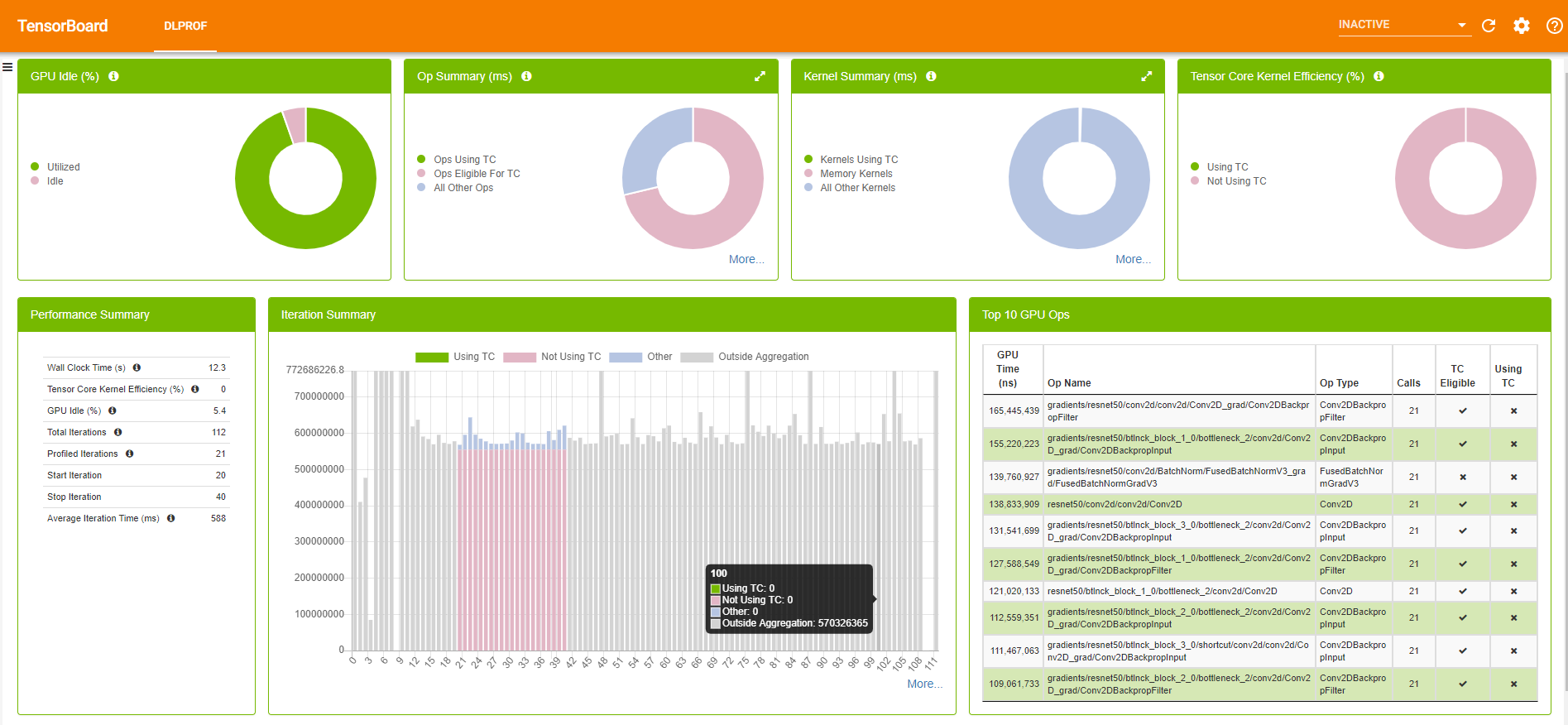
TensorBoard with the DLProf plugin has plenty of information about your model, ranging from the average time spent on iterations to the top 10 time-consuming kernels. For more information about the DLProf user interface, see the DLProf Plugin for TensorBoard User Guide.
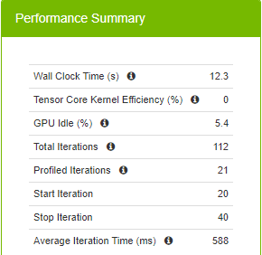
Figure 6 summarizes runtime metrics about the training. The total time spent for 20 iterations (the command defines starting at the 20th iteration and stopping at the 40th iteration) is 12.3 seconds, 588 ms for each iteration on average.
When you spend 588 ms on average for an iteration, you are not taking advantage of the new precision type, TF32, supported in A100. TF32 uses fewer bits in the matrix multiplications while providing the same model accuracy and therefore yields faster iterations. In addition to fewer bits to deal with, TF32 also makes use of Tensor Cores, which are specialized hardware for deep learning that help accelerate matrix multiply and accumulate operations. The Volta (V100), Turing (T4), and Ampere (A100) generations of GPUs have Tensor Cores.
TF32 is enabled by default in the NVIDIA NGC TensorFlow and PyTorch containers and is controlled with the NVIDIA_TF32_OVERRIDE=0 and NVIDIA_TF32_OVERRIDE=1 environment variables.
After enabling TF32, make the same call without changing any parameters. Figure 7 shows the top 10 GPU operations and if they are using Tensor Cores (TC).
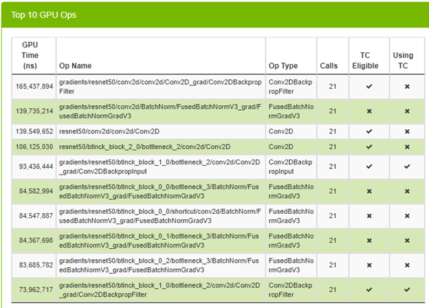
You can see that some operations are already using Tensor Cores, which is great. Look at the average time spent on an iteration to see if you have any speed up.
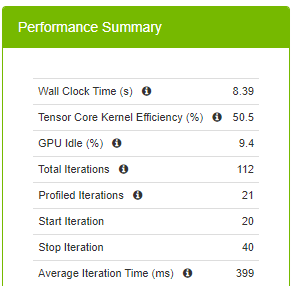
The average iteration time is reduced to 399 ms from 588 ms when you switch to the TF32 precision. This is a great speed up with switching one environment variable. The million-dollar question is whether you can do better than 399 ms. You know that you can do better than 588 ms, as DLProf makes this recommendation.
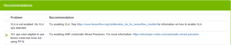
DLProf not only provides plenty of information about your model, it also makes suggestions on how you can improve it. In this case, it is suggesting that you enable XLA and AMP (automatic mixed precision). XLA is a linear algebra compiler targeting speeding up linear algebra operations. Numerical precision describes the number of digits that are used to express a value. Mixed precision combines different numerical precisions in a computational method. Deep learning networks can be trained with lower precision for high throughput, by halving storage requirements and memory traffic on certain tensors. Mixed precision accelerates training speed for large matrix to matrix multiply-add operations.
To enable XLA and AMP, set the following environment variables in a NVIDIA container:
export TF_XLA_FLAGS="--tf_xla_auto_jit=2"
export TF_ENABLE_AUTO_MIXED_PRECISION=1
That said, most of the recent repositories already have built-in support for XLA and AMP. What you usually must do is to pass related parameters. In this case, they were use_xla and use_tf_amp. After having XLA and AMP enabled, you can have your model use Tensor Cores efficiently, require less amount of memory, and take advantage of faster linear algebra operations.
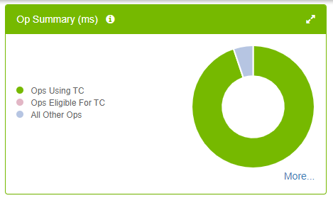
Figure 10 shows that almost all the Tensor Core–eligible operations are already using Tensor Cores (no pink slice in the pie chart). This is what you want to see. More importantly, it helps reduce the training time.
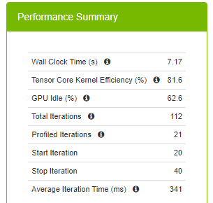
Average iteration time is reduced to 341 ms from 399 ms (and 588 ms). Using half precision yields less memory usage. To have a fair comparison, don’t change the batch size with mixed precision. That said, by enabling AMP, you could double the batch size for your model compared to full floating-point precision and it further reduces the training time.
To summarize, you first employed TF32 precision and reduced the training time. Then, you enabled AMP and XLA and further reduced the training time while using DLProf to help profile.
PyTorch and PyProf
In this section, we show you how to do profiling when creating models with PyTorch. We have already experienced several optimization techniques so far. Use TF32 and AMP for optimizing the model in PyTorch.
Here, you follow a more advanced path, where you inject some extra code to the code base. Further, you use PyProf and the Nsight Systems profiler directly, with no DLProf call. You can still use DLProf and TensorBoard for profiling PyTorch models, as DLProf supports PyTorch as well. However, we wanted to show you alternate ways of profiling.
You can cherry-pick what to profile, such as the 17th iteration only. In the data iteration loop, check to see if you are in the 17th iteration. If so, surround the lines that do the forward pass, loss calculation, gradient computation (backward), and update parameters (step) with the profiler start and stop markers.
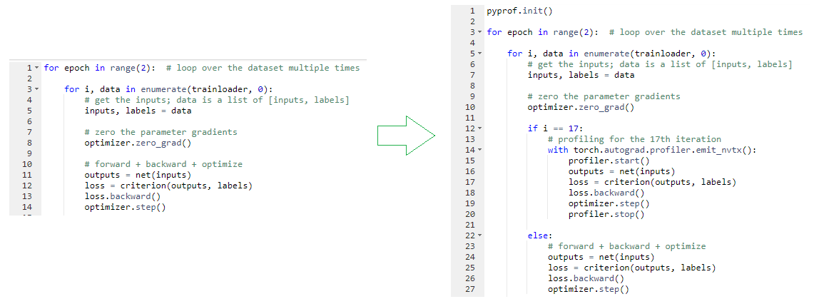
Borrow the ResNet50 training code from the same repo. Make the profiling changes in the training code and add the pyprof parameter to enable profiling for the only forward pass. You can leave the back propagation and set the range in any way you want, then push them to this branch for reference. With the changes, you make the call to run the PyTorch ResNet50 training along with profiling:
nsys profile --trace 'nvtx,cuda,osrt,cudnn' -c cudaProfilerApi --stop-on-range-end true \
--show-output true --sample=cpu --export=sqlite \
-o /ecan/pytorch_a100_profiling/resnet50_pytorch_fp32_b256 \
python main.py /ecan/imagenet_small \
--raport-file raport.json -j16 -p 100 --lr 2.048 \
--optimizer-batch-size 256 --warmup 8 --arch resnet50 \
 -c fanin --label-smoothing 0.1 \
 --lr-schedule cosine --training-only --mom 0.875 --wd 3.0517578125e-05 -b 256\
--epochs 1 --workspace /ecan/results \
--pyprof
This time, you call the Nsight Systems profiler directly. You already know the trace, sample, and output (-o) parameters. The -c cudaProfilerApi --stop-on-range-end true parameters are added to tell the profiler that you incepted start and stop markers so that the profiler profiles whatever happens only in between. When the --show-output parameter is set to true, the target process stdout and stderr streams are printed to the console.
This call resulted in two files: qdrep and sqlite. In TensorFlow, you used the event_files folder for TensorBoard but didn’t touch the qdrep file. This time, you use qdrep to inspect the profiling results visually in the Nsight Systems application.
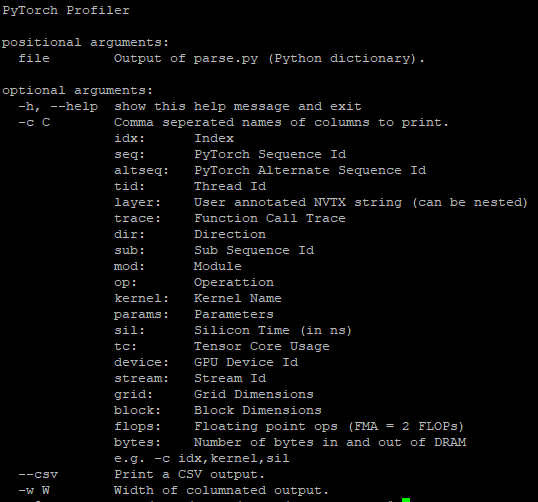
The following code example uses PyProf calls to analyze kernels:
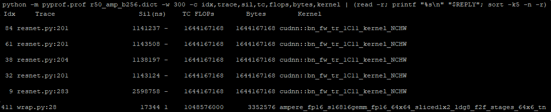
python -m pyprof.parse (resulting_sqlite_file_from_our_call) > a_file
python -m pyprof.prof a_file -w 100 -c idx,trace,sil,tc,flops,bytes,kernel \
| (read -r; printf “%s\n” “$REPLY”; sort -k5 -n -r)
The w parameter sets the column widths and the c parameter specifies the options to be printed out. There are several options and we have chosen these (see the complete list following). We also sorted by number of floating-point operations for a better analysis; otherwise, it is sorted in the order of execution.
We provide a few kernels from the top of the resulting list. The first few ones are batch normalization kernels. You can also identify the line number for a file in which it is called, for example, resnet50.py:201. This is useful for better understanding these kernel statistics, as there might be multiple batch normalizations in your model. The last row is a matrix multiplication using half precision. It is also using Tensor Cores, which is great.
Change the final line of the earlier PyProf call to obtain the total amount of nanoseconds that you spent on a forward pass of an iteration:
python -m pyprof.prof a_file -w 100 -c idx,trace,sil,tc,flops,bytes,kernel \
| awk ‘{total+=$3}END{print total}’
The result of the call is 188,388,811 ns (188.4 ms). Thus far, your profiling has been done using the FP32 precision type. You already know that switching to the TF32 precision type enables you to optimize your code. By toggling the NVIDIA_TF32_OVERRIDE environment variable, you can take advantage of the TF32 precision type.
When you have the same training and profiling calls but with the TF32 precision type enabled this time, you get a total time of 110,250,534 ns (110.25 ms). By switching to TF32, you almost halved the execution time.
You got used to doing optimization on TensorFlow, and now you are optimizing code on PyTorch. You have one more step to go: Enable mixed precision and see if you can further optimize your code.
nsys profile --trace 'nvtx,cuda,osrt,cudnn' -c cudaProfilerApi --stop-on-range-end true \
--show-output true --sample=cpu --export=sqlite \
-o /ecan/pytorch_a100_profiling/resnet50_pytorch_amp_b256 \
python main.py /ecan/imagenet_small \
--raport-file raport.json -j16 -p 100 --lr 2.048 \
 --optimizer-batch-size 256 --warmup 8 --arch resnet50 \
 -c fanin --label-smoothing 0.1 \
 --lr-schedule cosine --training-only --mom 0.875 --wd 3.0517578125e-05 -b 256 \
--amp --static-loss-scale 128 \
--epochs 1 --workspace /ecan/results \
--pyprof
Most of the parameters are the same as the previous call except the amp and static-loss-scale parameters. The amp parameter enables AMP as the code base supports it. The static-loss-scale parameter scales the loss. For more information about ResNet50 training parameters, see the Command-line options section in the ResNet50 v1.5 For PyTorch guide.
When you run the code example for the call with AMP mode on, you get 72,860,695 ns (72.86 ms). This is wonderful news, as you further optimized your code using mixed precision. You get similar improvements on TensorFlow. Even though TensorFlow has an extra optimization (XLA), you get further improvements on PyTorch with only AMP.
Nsight Systems for profiling
So far, you have used the statistics harvested from training with the profiler call. You have also made use of PyProf to take a quick peek at the kernels used in the model. You produced great visualizations using TensorBoard and the DLProf plugin. In the beginning of the post, you used nvidia-smi to check the GPU utilization. If you think these are not enough and you want to dive deeper, no worries. We have more for you.
The qdrep files are obtained when training with the profiler call is completed. Now it is time to use them to analyze your model more deeply using the user interface of the NVIDIA Nsight Systems profiler. For more information, see the Nsight Systems User Guide.
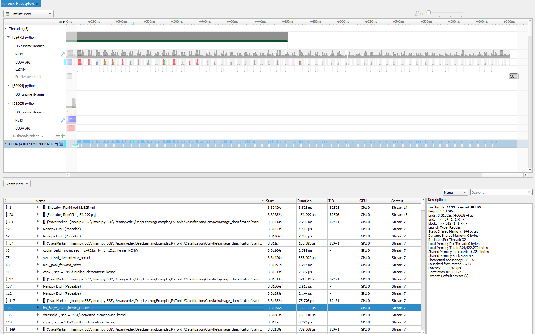
Even if you limit profiling to forward propagation of an iteration only, with the Nsight Systems profiler you can inspect lots of information visually. We sometimes zoom in to a particular region from this view to further analyze. To get a closer look, zoom into the beginning of the training, focused on a few milliseconds.
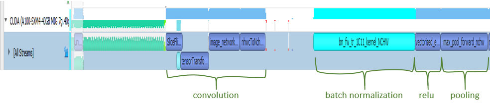
You first see some memory operations in green, which is followed by the convolution operation. Then, batch normalization kicks in. Not surprisingly, an activation function is the next step. In this case, it is ReLU. Finally, you see that max pooling is executed. This is the order that you see in the code base and in most of the ResNet models. You can also see stack trace for more information for selected operations, which become turquoise green when selected.
Before we end this post, we would like to show yet another optimization method. In PyTorch, you can also change the memory format. Data is usually stored in the following format:
[ number of elements in the batch, number of channels (depth or number of filters), height, width ]
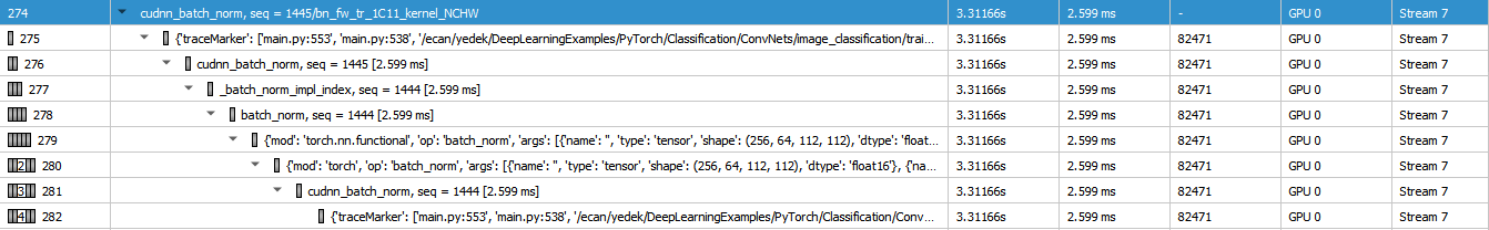
That said, PyTorch operates on the [n, h, w, c] format. The batch-norm like layers are processed faster in the [n, h, w, c] format. The most time-consuming operations were batch normalization (as in Figure 14). Furthermore, Tensor Cores natively use the [n, h, w, c] format. Basically, by changing the memory format, you can save some time while processing batch-norm–like layers as well as avoiding some format conversion time inside the CUDNN kernels.
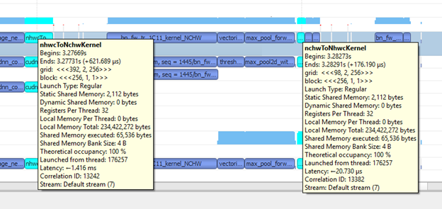
Adding --memory format nchw to the earlier call does the trick and enables you to use the [n, c, h, w] memory format. With the [n, c, h, w] memory format, your training no longer needs memory format conversion operations, for example, nhwcToNchwKernel and nchwToNhwcKernel (see Figure 18). This means that you saved some more time. In other words, you did yet another optimization by changing the memory format. Just to confirm this, calculate the total amount of time spent on kernels. For us, it turned out to be 45,631,828 ns (45.6 ms). It was around 70 ms with the [n, c, h, w] memory format. You further cut your execution time with the memory format optimization technique.
Summary
This post covered the details of profiling deep learning models using a variety of tools: nvidia-smi, DLProf and PyProf, and the NVIDIA Nsight Systems profiler. Each tool is useful to point out performance improvement opportunities at different levels. The profiling runs used two common deep learning frameworks: PyTorch and TensorFlow. The code examples are provided in the DeepLearningExamples GitHub repo, which also has the code changes for the PyProf and PyTorch calls. We encourage you to replicate these steps to get more familiar with the profiling tools.
For more information, see the following resources:
Acknowledgements
Thanks to David Zier, Timothy Gerdes, Elias Bermudez, Matthew Kotila, and Ujval Kapasi for their continued support throughout the progress of this post.