5G 和 6G 的发展需要高保真无线电信道建模,但当前生态系统高度分散。链路级模拟器、网络级模拟器与 AI 训练框架通常采用不同的编程语言,独立运行。
如果您是致力于模拟 5G 或 6G 系统物理层关键组件行为的研究人员或工程师,本教程将指导您如何扩展仿真链路,并集成由 Aerial Omniverse 数字孪生 (AODT) 生成的高保真信道模型。
预备知识:
- 硬件: NVIDIA RTX GPU(建议采用 Ada 架构或更新架构以获得更优性能)。
- 软件: 访问 AODT 版本 1.4 容器。
- 知识: 基本熟悉 Python 及无线网络概念,例如无线电单元(RU)和用户设备(UE)。
AODT 通用嵌入式服务架构
图 1 展示了如何将 AODT 嵌入到任意仿真链中,无论该仿真链使用的是 C++、Python 还是 MATLAB。

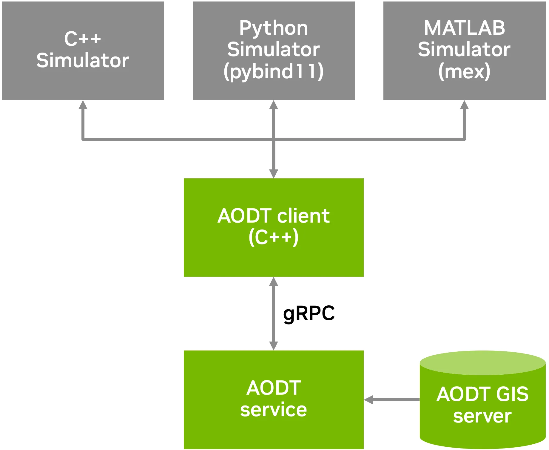
AODT 分为两个主要组成部分:
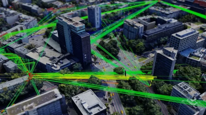
- AODT 服务充当集中式、高功率计算核心,负责管理和加载大型 3D 城市模型(例如来自 Omniverse Nucleus 服务器的模型),并执行所有复杂的电磁(EM)物理计算。
- AODT 客户端及语言绑定提供轻量级的开发者接口,客户端处理全部服务调用,并通过 GPU IPC 高效传输数据,实现对无线电信道输出的直接 GPU 显存访问。为支持广泛的开发环境,AODT 客户端提供通用语言绑定,可直接用于 C++、Python(通过
pybind11)以及 MATLAB(通过用户实现的mex)。
工作流程的实际应用:通过 7 个简单步骤计算信道脉冲响应
那么,您实际将如何使用它呢?整个工作流程设计简洁,遵循由客户端编排的精确序列,如图 3 所示。

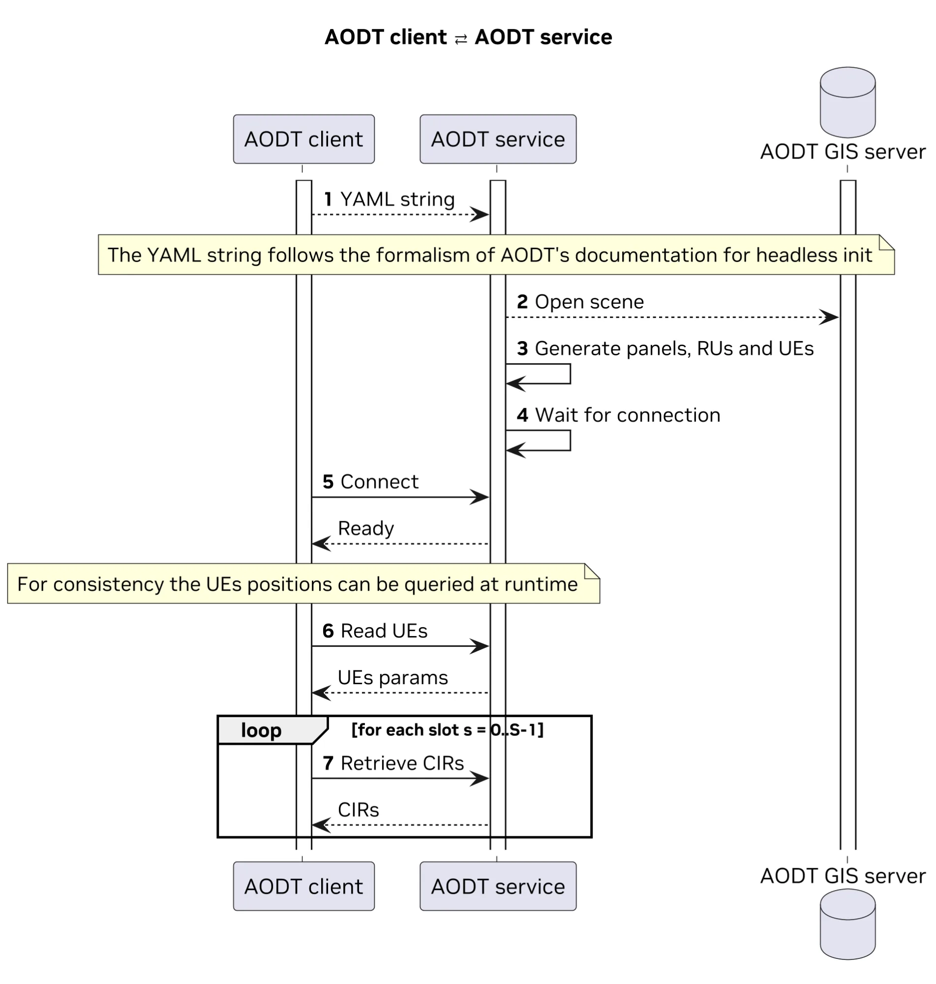
该过程分为两个主要阶段:
- 配置指定 AODT 要模拟的内容。
- 执行运行仿真以获取数据。
请遵循完整示例:
第 1 阶段:配置 (构建 YAML 字符串)
AODT 服务通过单个 YAML 字符串进行配置。您可手动编写该字符串,同时也可使用功能强大的 Python API 来以编程方式逐步构建配置内容。
第 1 步。初始化仿真配置
首先,导入配置对象并设置基本参数:要加载的场景、仿真模式(例如 SimMode.EM)、要运行的插槽数,以及用于生成可重复且确定性结果的种子。
from _config import (SimConfig, SimMode, DBTable, Panel)

# EM is the default mode.
config = SimConfig(scene, SimMode.EM)

# One batch is the default.
config.set_num_batches(1)

config.set_timeline(
    slots_per_batch=15000,
    realizations_per_slot=1
)

# Seeding is disabled by default.
config.set_seed(seed=1)
config.add_tables_to_db(DBTable.CIRS)
第 2 步:定义天线阵列
接下来,为基站(RU)和用户设备(UE)定义天线面板。可以采用如 ThreeGPP38901 等标准模型,也可自定义模型。
# Declare the panel for the RU
ru_panel = Panel.create_panel(
    antenna_elements=[AntennaElement.ThreeGPP38901],
    frequency_mhz=3600,
    vertical_spacing=0.5,
    vertical_num=1,
    horizontal_spacing=0.5,
    horizontal_num=1,
    dual_polarized=True,
    roll_first=-45,
    roll_second=45)

# Set as default for RUs
config.set_default_panel_ru(ru_panel)

# Declare the panel for the UE
ue_panel = Panel.create_panel(
    antenna_elements=[AntennaElement.InfinitesimalDipole],
    frequency_mhz=3600,
    vertical_spacing=0.5,
    vertical_num=1,
    horizontal_spacing=0.5,
    horizontal_num=1,
    dual_polarized=True,
    roll_first=-45,
    roll_second=45)

# Set as default for UEs
config.set_default_panel_ue(ue_panel)
第 3 步:部署网络组件(RU 和手动 UE)
将网络元素置于场景中,我们采用地理参考坐标(纬度/经度)进行精确定位。对于 UE,可定义一系列路标以生成预设路径。
du = Nodes.create_du(
      du_id=1,
      frequency_mhz=3600,
      scs_khz=30
	)

ru = Nodes.create_ru(
    		ru_id=1,
      	frequency_mhz=3600,
    		radiated_power_dbm=43,
    		du_id=du.id,
	)


ru.set_position(
	Position.georef(
     		35.66356389841298,
        	139.74686323425487))


ru.set_height(2.5)
ru.set_mech_azimuth(0.0)
ru.set_mech_tilt(10.0)


ue = Nodes.ue(
    		ue_id=1,
   		radiated_power_dbm=26,
	)


ue.add_waypoint(
	Position.georef(
       	35.66376818087683,
       	139.7459968717682))
ue.add_waypoint(
    Position.georef(
       	35.663622296081414,
        	139.74622811587614))
ue.add_waypoint(
    Position.georef(
        	35.66362516562424,
        	139.74653110368598))

config.add_ue(ue)
config.add_du(du)
config.add_ru(ru)
第 4 步:部署动态元素(程序化生成与散布器)
这就是仿真真正变得动态的地方。您可以定义 spawn_zone,让 AODT 在该区域内程序化地生成具有逼真移动行为的 UE,而无需手动放置每一个 UE。此外,您还可以启用 urban_mobility,以引入动态散射器(如汽车),这些散射器能与无线电信号发生物理交互并影响信号传播。
# If we want to enable procedural UEs we need a spawn zone.
config.add_spawn_zone(
	translate=[150.2060449, 99.5086621, 0],
    	scale=[1.5, 2.5, 1],
    	rotate_xyz=[0, 0, 71.0])

# Procedural UEs are zero by default.
config.set_num_procedural_ues(1)

# Indoor proc. UEs are 0% by default.
config.set_perc_indoor_procedural_ues(0.0)

# Urban mobility is disabled by default.
config.enable_urban_mobility(
	vehicles=50,
    	enable_dynamic_scattering=True)

# Save to string
from omegaconf import OmegaConf
config_dict = config.to_dict()yaml_string = OmegaConf.to_yaml(config_dict)
第 2 阶段:执行 (客户端 – 服务器交互)
现在我们有了 yaml_string 配置,便可以连接到 AODT 服务并运行仿真。
第 5 步:连接
导入 dt_client 库,创建指向服务地址的客户端,并调用 client.start(yaml_string)。通过这一调用,可将完整配置发送至服务端,随后服务将加载 3D 场景、生成所有对象并准备仿真。
import dt_client
import numpy as np
import matplotlib.pyplot as plt

# Server address (currently only localhost is supported)
server_address = "localhost:50051"

# Create client
client = dt_client.DigitalTwinClient(server_address)

try:
    client.start(yaml_string)
except RuntimeError as e:
    print(f"X Failed to start scenario: {e}")
    return 1
启动后,您可以查询服务以获取刚刚创建的仿真参数,从而确认一切已准备就绪,并了解预期的插槽、RU 和 UE 数量。
try:
    	status = client.get_status()
    	num_batches = status['total_batches']
    	num_slots = status['slots_per_batch']
     	num_rus = status['num_rus']
    	num_ues = status['num_ues']
except RuntimeError as e:
    	print(f"X Failed to get status: {e}")
    	return 1
第 6 步:获取 UE 位置
for slot in range(num_slots):
	try:
     		ue_positions = client.get_ue_positions(batch_index=0,
            	temporal_index=SlotIndex(slot))
    	except RuntimeError as e:
        	print(f"X Failed to get UE pos: {e}")
第 7 步:检索通道脉冲响应
现在,我们遍历每个模拟插槽,可以在其中获取所有 UE 的当前位置。这对于验证移动模型是否按预期运行,以及将信道数据与位置信息关联起来至关重要。
检索核心仿真数据是至关重要的一步。通道脉冲响应 (CIR) 描述了信号如何从每个 RU 传播到每个 UE,包括所有多路径组件 (其延迟、振幅和相位)。
为/ 从/at 检索大量数据?每个插槽都会变慢。为加快速度,API 采用 IPC 的零复制两步流程。
首先,在循环开始前,您需要请求客户端为 CIR 结果分配 GPU 显存。该服务将执行此操作,并返回一个 IPC 句柄,即指向该 GPU 显存的指针。
ru_indices = [0]
ue_indices_per_ru = [[0, 1]]
is_full_antenna_pair = False

try:
    # Step 1: Allocate GPU memory for CIR
    cir_alloc_result = client.allocate_cirs_memory(
            	ru_indices,
            	ue_indices_per_ru,
            	is_full_antenna_pair)

    	values_ipc_handles = cir_alloc_result['values_handles']
    	delays_ipc_handles = cir_alloc_result['delays_handles']
现在,在循环中,您可以调用 client.get_cirs(…),并传入这些内存句柄。AODT 服务会为该插槽执行完整的 EM 模拟,并将结果直接写入共享的 GPU 显存中,无需通过网络复制任何数据,因此效率非常高。客户端将立即收到通知,表明新数据已准备就绪。
# Step 2: Retrieve CIR
    	cirs = client.get_cirs(
            	values_ipc_handles,
            	delays_ipc_handles,
            	batch_index=0,
           	temporal_index=SlotIndex(0),
            	ru_indices=ru_indices,
            	ue_indices_per_ru=ue_indices_per_ru,
            	is_full_antenna_pair=is_full_antenna_pair)

    values_shapes = cirs['values_shapes']
    delays_shapes = cirs['delays_shapes']
访问 NumPy 中的数据
数据(CIR 值和延迟)仍驻留在 GPU 上。客户端库提供了简单的实用工具,可获取 GPU 指针,同时避免引入额外延迟。为便于使用,也支持通过 NumPy 访问这些数据,具体可通过以下代码实现。
 # Step 3: export to numpy
	for i in range(len(ru_indices)):
     		values_gpu_ptr = client.access_values_gpu(
                values_ipc_handles[i],
                values_shapes[i])
        	delays_gpu_ptr = client.access_delays_gpu(
                	delays_ipc_handles[i],
                	delays_shapes[i])
        	values = client.gpu_to_numpy(
                	values_gpu_ptr,
                	values_shapes[i])
        	delays = client.gpu_to_numpy(
                delays_gpu_ptr,
                delays_shapes[i])
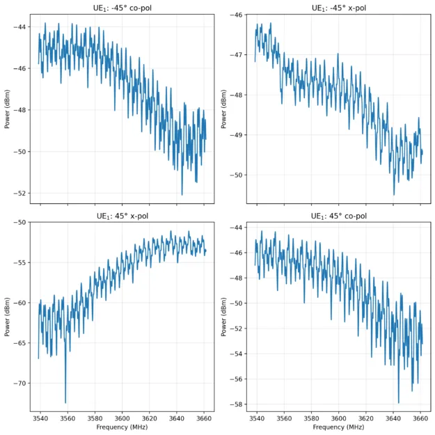
就是这样!仅用几行 Python 代码,您便已配置了一个复杂、动态且具备地理参考的模拟,该模拟将在功能强大的远程服务器上运行,并将基于物理特性的高保真 CIR 以 NumPy 数组的形式返回。现在,这些数据可用于可视化、分析,或直接输入到 AI 训练管线中。例如,我们可以利用以下图形函数,可视化前述手动声明的 UE 频率响应。
def cfr_from_cir(h, tau, freqs_hz):
    	phase_arg = -1j * 2.0 * np.pi * np.outer(tau, freqs_hz)

    	# Safe exponential and matrix multiplication
    	with np.errstate(all='ignore'):
        	# Sanitize inputs
        	h =  np.where(np.isfinite(h), h, 0.0)

        	expm = np.exp(phase_arg)
        	expm = np.where(np.isfinite(expm), expm, 0.0)

           result = h @ expm
        	result = np.where(np.isfinite(result), result, 0.0)

    	return result

def plot(values, delays):
# values shape:
# [n_ue,     number of UEs
#  n_symbol, number of OFDM symbols
#  n_ue_h,   number of horizontal sites in the UE panel
#  n_ue_v,   number of vertical sites in the UE panel
#  n_ue_p,   number of polarizations in the UE panel
#  n_ru_h,   number of horizontal sites in the RU panel
#  n_ru_v,   number of vertical sites in the RU panel
#  n_ru_p,   number of polarizations in the RU panel
#  n_tap     number of taps
# ]
AX_UE, AX_SYM, AX_UEH, AX_UEV, AX_UEP, AX_RUH, AX_RUV, AX_RUP,AX_TAPS = range(9)
# delays shape:
# [n_ue,      number of UEs
#  n_symbols, number of OFDM symbols
#  n_ue_h,    number of horizontal sites in the UE panel
#  n_ue_v,    number of vertical sites in the UE panel
#  n_ru_h,    number of horizontal sites in the RU panel
#  n_ru_v,    number of vertical sites in the RU panel
#  n_tap      number of taps
# ]
D_AX_UE, D_AX_SYM, D_AX_UEH, D_AX_UEV, D_AX_RUH, D_AX_RUV, D_AX_TAPS = range(7)

nbins = 4096
    	spacing_khz = 30.0
     	freqs_hz = (np.arange(nbins) - (nbins // 2)) * \
spacing_khz * 1e3

    	# Setup Figure (2x2 grid)
fig, axes = plt.subplots(nrows=2, ncols=2, figsize=(8, 9), \
sharex=True)
    	axes = axes.ravel()

cases = [(0,0), (0,1), (1,0), (1,1)]
    	titles = [
        	"UE$_1$: -45° co-pol",
        	"UE$_1$: -45° x-pol",
        	"UE$_1$: 45° x-pol",
        	"UE$_1$: 45° co-pol"
    	]

    	for ax, (j, k), title in zip(axes, cases, titles):
     		try:
     		# Construct index tuple: [i, 0, 0, 0, j, 0, 0,
# k, :]
           idx_vals = [0] * values_full.ndim
           idx_vals[AX_UE] = i_fixed
           idx_vals[AX_UEP] = j  # UE polarization
           idx_vals[AX_RUP] = k  # RU polarization
           idx_vals[AX_TAPS] = slice(None) # All taps

           h_i = values_full[tuple(idx_vals)]
           h_i = np.squeeze(h_i)

           # Construct index tuple: [i, 0, 0, 0, 0, 0, :]
           idx_del = [0] * delays_full.ndim
           idx_del[D_AX_UE] = i_fixed
           idx_del[D_AX_TAPS] = slice(None)

           tau_i = delays_full[tuple(idx_del)]
           tau_i = np.squeeze(tau_i) * DELAY_SCALE

           H = cfr_from_cir(h_i, tau_i, freqs_hz)

           power_w = np.abs(H) ** 2
           power_w = np.maximum(power_w, 1e-12)
           power_dbm = 10.0 * np.log10(power_w) + 30.0

           ax.plot(freqs_hz/1e6 + 3600, power_dbm, \
linewidth=1.5)
           ax.set_title(title)
           ax.grid(True, alpha=0.3)

   	# Formatting
for ax in axes:
    		ax.set_ylabel("Power (dBm)")

    	axes[2].set_xlabel("Frequency (MHz)")
    	axes[3].set_xlabel("Frequency (MHz)")

    	plt.tight_layout()
    	plt.show()

助力 AI 原生 6G 时代
从 5G 到 6G 的过渡必须应对无线信号处理中日益复杂的问题,其特点是数据量庞大、异质性显著,以及 AI 原生网络成为核心任务。传统的孤立模拟方法难以胜任这一挑战。
NVIDIA Aerial Omniverse 数字孪生专为这一新时代而打造。通过在版本 1.4 中迁移到基于 gRPC 的服务架构,AODT 正在推动基于物理的无线电仿真普及,并为机器学习与算法探索提供所需的地面实况数据。
AODT 1.4 可在 NVIDIA NGC。我们诚邀研究人员、开发者和运营商集成这一强大的新服务,携手共建 6G 的未来。