为了获得最先进的机器学习( ML )解决方案,数据科学家通常建立复杂的 ML 模型。然而, 这些技术的计算成本很高,直到最近还需要广泛的背景知识、经验和人力。
最近,在 GTC21 , AWS 高级数据科学家 尼克·埃里克森 给出了一个 session 分享如何结合 AutoGluon , RAPIDS 和 NVIDIA GPU 计算简化实现最先进的 ML 精度,同时提高性能和降低成本。 这篇文章概述了尼克会议的一些要点:
- AutoML 是什么? AutoGluon 有什么不同?
- 在 Kaggle 预测比赛中, AutoGluon 如何在仅仅三行代码的情况下就超过 99% 的人类数据科学团队, 不需要专家知识?
- AutoGluon 与 RAPIDS 的集成如何使训练速度提高 40 倍,推理速度提高 10 倍?
什么是AutoGluon?
AutoGluon 是一个开放源代码的 AutoML 库,它支持易于使用和易于扩展的 AutoML ,重点放在自动堆栈合并、深度学习和跨文本、图像和表格数据的真实应用程序上。面向 ML 初学者和专家, AutoGluon 使您能够:
- 用几行代码为您的原始数据快速构建深度学习和经典 ML 解决方案的原型。
- 在没有专家知识的情况下自动使用最先进的技术(如适用)。
- 利用自动超参数调整、模型选择/装配、架构搜索和数据处理。
- 轻松改进/调整您的定制模型和数据管道,或为您的用例定制 AutoGluon 。
本文主要关注 AutoGluon Tabular ,这是一个 AutoGluon API ,它只需要几行 Python 就可以在未处理的表格数据集(如 CSV 文件)上训练高度精确的机器学习模型。 为了理解 AutoGluon Tabular 是如何做到这一点的,我们将首先解释一些概念。
什么是监督机器学习?
有监督机器学习 将一组带标签的训练实例作为输入,并构建一个模型,该模型旨在基于我们知道的关于该实例的其他信息(称为实例的特征)正确预测每个训练实例的标签。这样做的目的是建立一个精确的模型,可以自动用未知的标签标记未来的数据。

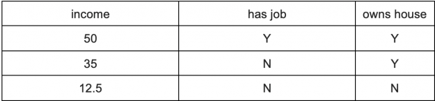
在表格数据集中,列表示变量的度量(又称特征),行表示单个数据点。 例如,下表显示了一个包含三列的小数据集:“有工作”、“拥有房子”和“收入”。在本例中,“ income ”是标签(有时称为预测的目标变量),其他列是用于尝试预测收入的特征。
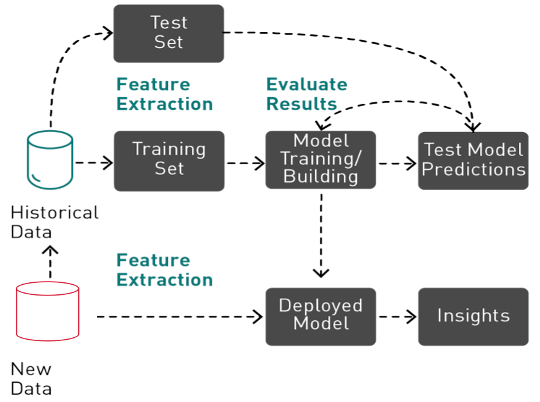
有监督机器学习是一个迭代的、探索性的过程,它涉及到数据准备、特征工程、验证拆分、缺失值处理、训练、测试、超参数调整、集成和评估 ML 模型,然后才能将模型用于生产中进行预测。
什么是 AutoML
历史上,实现最先进的 ML 性能需要广泛的背景知识、经验和人力。根据自动化的工具和级别, AutoML 使用不同的算法技术来尝试为 ml 管道找到最佳的特性、超参数、算法和/或算法组合。通过 automating 耗时的 ML 管道,从业者和企业可以应用机器学习更快更容易地解决业务问题。
AutoML 分三步进行, AutoGluon 表格
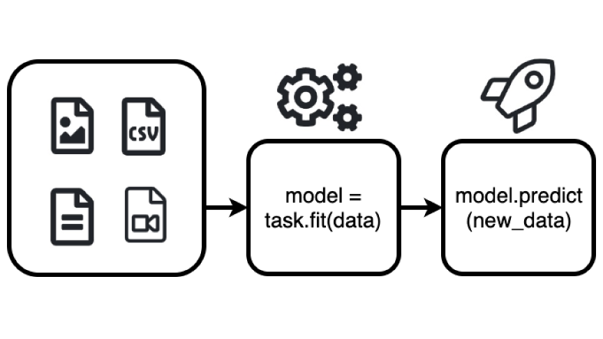
自动胶合板 可用于自动构建最先进的模型,该模型使用两个函数 fit () 和 predict () 根据同一行中的其他列预测特定列的值,如下所示。
from autogluon.tabular import TabularPredictor, TabularDataset
# load dataset
train_data = TabularDataset(DATASET_PATH)
# fit the model
predictor = TabularPredictor(label=LABEL_COLUMN_NAME).fit(train_data)
# make predictions on new data
prediction = predictor.predict(new_data)
函数的作用是:研究数据集,执行数据预处理,拟合多个模型,并将它们结合起来生成一个高精度的模型。有关要尝试的更完整的示例,请参见 关于预测表中列的 AutoGluon 快速入门教程。
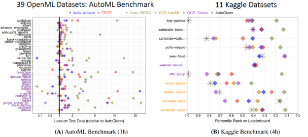
用这个简单的代码, AutoGluon 击败了其他 AutoML 框架和许多顶尖的数据科学家。 广泛的评估 通过对 Kaggle 和 OpenML AutoML 基准测试的 50 个分类和回归任务进行测试,发现 AutoGluon 比 TPOT 、 H2O 、 AutoWEKA 、 AutoSklearn 和 Google AutoML 表更快、更健壮、更准确。同样在两个受欢迎的 Kaggle 比赛中, AutoGluon 在仅仅 4 小时的原始数据训练后就击败了 99% 的数据科学家。
自粘胶有什么不同?
大多数 AutoML 框架致力于将算法选择和超参数优化( CASH )结合起来,提供从各种可能性中寻找最佳模型及其超参数的策略。然而,现金有一些缺点:
- 它需要许多重复的模型训练,而且大多数模型都被丢弃了,而没有对最终结果做出贡献。
- 超参数调优做得越多,验证数据拟合过度的风险就越高。
- 超参数调整在加密时不太有用。
相比之下, AutoGluon Tabular 依靠专家数据科学家使用的方法来赢得竞争:将多个模型集合起来,并将它们堆叠在多个层中,从而优于其他框架。
Ensembling 是如何工作的?
集成学习方法结合多种机器学习( ML )算法来获得更好的模型。为了更好地理解这一点,让我们看看随机森林,它是决策树的集合。
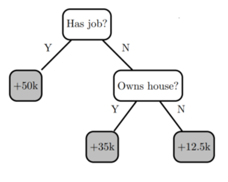
决策树通过评估 if-then-else 和真/假特征问题树,并估计评估做出正确决策的概率所需的最小问题数,创建预测目标标签的模型。决策树可用于分类以预测类别,或用于回归以预测连续数值。例如,下面的决策树(基于上表)尝试使用特征“ has job ”和“ owns house ”的两个决策节点来预测标签“ income ”。
决策树的优点是易于解释,但存在过度拟合和准确性问题。建立一个精确的模型是介于两者之间的 以及过度拟合——模型预测与训练数据的行为方式相匹配,并且被广泛化,足以对看不见的数据进行准确预测。
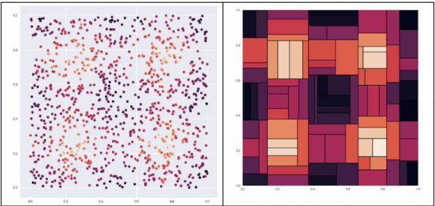
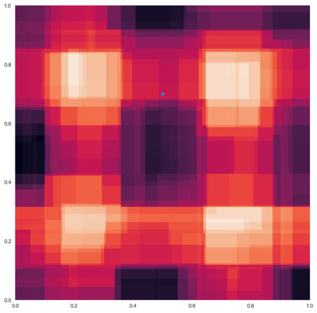
决策树试图找到最佳分割来对数据进行子集划分,这会导致严重的分割。 例如,给定下面左边的数据集,我们想预测一个点的颜色,点越亮,值就越高。如右图所示,决策树会将数据分割成多个块。 下一步,我们将研究如何使用 ensembling 改进决策树。
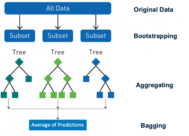
Ensembling 是一种通过组合预测和改进泛化来提高模型精度的行之有效的方法。 随机森林 是一种流行的分类和回归集成学习方法。 Random forest 使用一种称为 bagging ( bootstrap aggregating )的技术,从数据集和特征的随机 bootstrap 样本并行地构建完整的决策树。 通过对所有树的输出进行聚合来进行预测,减少了方差,提高了预测精度。最终的预测是所有决策树预测的多数类或均值回归。 随机性对森林的成功至关重要, bagging 确保没有决策树是相同的,减少了单个树的过度拟合问题。
为了理解这是如何给出更好的预测,让我们看一个例子。这里是图 6 中所示的数据集的四个不同的决策树,测试数据点的预测颜色不同。我们可以看到,每一种方法都给出了解的近似值,而这种近似值不足以作出精确的预测。
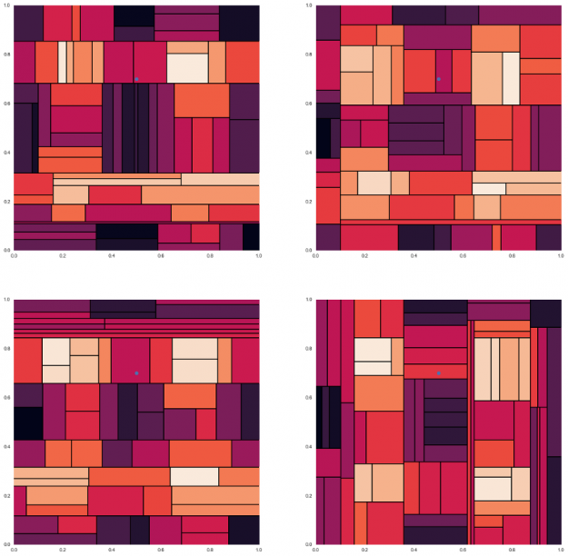
图像参考 https :// gist . github . com / tylerwx51 / fc8b316337833c877785222d463a45b0
当这四个决策树被合并并平均在一起时,粗糙的边界消失了,并且像下面的随机森林示例一样被平滑。现在 测试数据点的预测颜色是来自其他树预测的颜色的混合。
随机林中的所有决策树都是次优的,它们在随机方向上都是错误的。当平均决策树时,它们错误的原因相互抵消,这称为方差抵消。 结果质量更高,因为它们反映了大多数树做出的决定。平均值限制了误差,即使有些树是错的,有些树是对的,所以这组树一起朝着正确的方向移动。
当许多不相关的决策树组合在一起时,它们产生的模型具有很高的预测能力,能够抵抗过度拟合。这些概念是流行的机器学习算法的基础,例如 随机森林, XGBoost , Catboost 和 LightGBM 这些都是由自动胶所使用的。
多层叠加
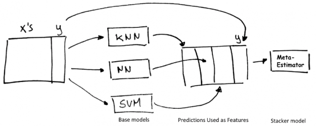
你可以更进一步与 ensembling ,经验丰富的机器学习实践者 将 RandomForest 、 CatBoost 、 k 近邻和其他的输出结合起来,以进一步提高模型精度。在 ML 竞争社区很难找到一个单一的模型赢得的竞争,每一个获胜的解决方案都包含了模型的集合。
Stacking 是一种使用“基本”回归或分类模型集合的聚合预测作为训练元分类器或回归“堆栈”模型的特征的技术。
多层堆垛机将堆垛机模型输出的预测结果作为输入输入到其他更高层的堆垛机模型中。在许多 Kaggle 比赛中,在多个层次上迭代这个过程是一个获胜的策略。多层叠加集成功能强大,但很难使用和实现,目前除了 Autogluon 之外,其他任何 AutoML 框架都没有使用它。
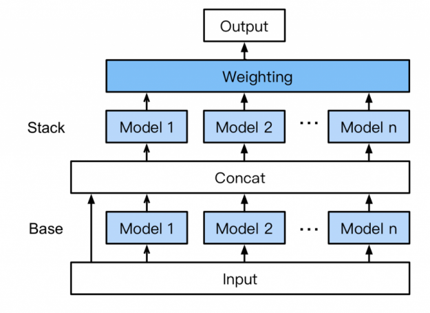
无需专家知识, AutoGluon 自动组装和训练一种新形式的多层堆叠,如图 11 所示,采用 k 折叠装袋。其工作原理如下:
- 底座: 第一层有多个基础模型,这些模型分别经过训练,并使用 k-fold 集成装袋(下文讨论)。
- 连接:将基础层模型预测与输入特征连接起来,作为下一层的训练输入。
- 堆垛:多个堆垛机模型在 concat 层输出上进行训练。与传统的堆叠策略不同, AutoGluon 重用与 stackers 相同的基本层模型类型(具有相同的超参数值)。 此外,堆垛机模型不仅将前一层模型的预测作为输入,而且还将原始数据特征本身作为输入。
- 加权:最后的堆叠层应用集合选择以加权的方式聚合堆叠机模型的预测。 在高容量模型堆栈中聚合预测可以提高对过度拟合的恢复能力
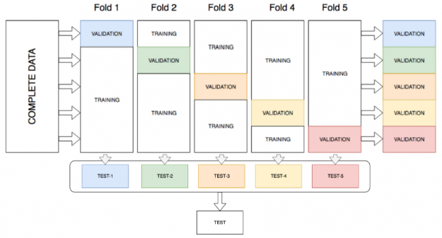
k-fold Ensembling 套袋
AutoGluon 通过将所有可用数据用于训练和验证,通过在堆栈的所有层对所有模型进行 k 折集成装袋来提高堆栈性能。 k-fold ensemble bagging 类似于 k-fold cross validation,这是一种最大化训练数据集的方法,通常用于超参数调整以确定最佳模型参数。通过 k 折交叉验证,数据被随机分成 k 个分区(折叠)。每个折叠一次用作验证数据集,而其余的 (Out-Of-Fold – OOF) 用于训练。模型使用 OOF 训练集进行训练并使用验证集进行评估,从而产生 k 个模型精度测量值。 AutoGluon 不是确定最佳模型并丢弃其余模型,而是将所有模型打包并从训练期间未看到的分区上的每个模型获得 OOF 预测。这为每个模型创建了 k 折预测,用作下一层的元特征。
为了进一步提高预测精度和减少过度拟合, AutoGluon 表格 在训练数据的 n 个不同的随机分区上重复 k 次装袋过程,平均重复袋子上的所有 OOF 预测。在调用 fit ()函数时,通过估计在指定的时间限制内可以完成多少轮来选择 n 。
为什么 AutoGluon 需要 GPU 加速
多层堆栈集成提高了精度,然而,这意味着要训练数百个模型,这比基本的 ML 用例需要更多的计算密集型任务,并且比加权集成要贵 10 到 20 倍。 在过去,复杂性和计算需求使得多层堆栈集成很难在许多生产用例和大型数据集上实现。对于 AutoGluon 和 NVIDIA GPU 计算 ,情况不再如此。
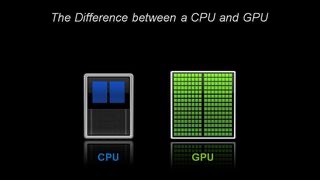
在体系结构上, CPU 由几个内核组成,这些内核有大量的高速缓存,一次可以处理几个软件线程。相反, GPU 由数百个内核组成 可以同时处理数千个线程。 GPU 的性能超过 20 倍 在 ML 工作流程中比 CPU 更快,并彻底改变了深度学习领域。
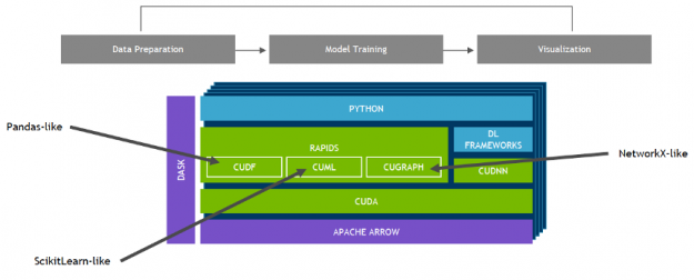
NVIDIA 开发了 RAPIDS ——一个开源的数据分析和机器学习加速平台,用于在 GPUs 中完全执行端到端的数据科学培训管道。它依赖于 NVIDIA ® [[ZCK0 号]® 用于低级计算优化的原语,但通过用户友好的 Python 接口(如 pandas 和 sciketlearnapi )公开了 GPU 并行性和高内存带宽。
使用 RAPIDS 的 cuML , 流行的机器学习算法,比如随机森林, XGBoost 和其他许多产品都支持单 GPU 和大型数据中心部署。对于大型数据集,这些基于 GPU 的实现可以加快机器学习模型的训练速度—通过 在随机森林的情况下高达 45 倍 ,超过 100x 支持向量机 和 k 近邻最高可达 600 倍 。这些加速可以将夜间作业转换为交互式作业,允许探索更大的数据集,并且可以在以前训练单个模型所需的时间内尝试几十种模型变体。
AutoGluon 的 最新版本 通过与 RAPIDS 集成,充分利用了 NVIDIA GPU 计算的潜力。通过这些集成, AutoGluon 能够在 GPU 上训练流行的 ml 算法并提高性能, 使更广泛的受众能够访问高性能的 AutoML 。
AutoGluon + RAPIDS 基准
对于 1 . 15 亿行航空公司数据集 用于梯度增压机 ( GBM ) 基准测试套件 , AutoGluon + RAPIDS 的训练速度比 cpu 上的 AutoGluon 快 25 倍,准确率为 81 . 92% ,比 XGBoost 基线高 7% 。 GPU 更喜欢更长的培训时间,因为固定的启动成本变得不那么重要。
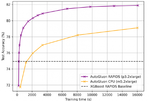
为了获得 81 . 92% 的准确率, gpu 上的 AutoGluon + RAPIDS 训练时间为 4 小时,而 cpu 为 4 . 5 天。
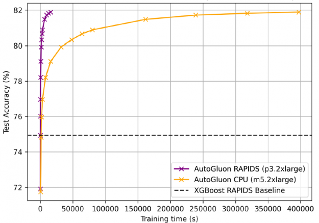
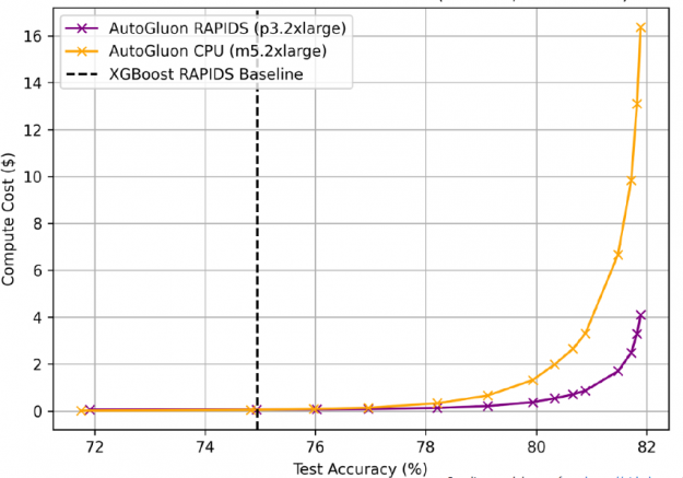
GPU 上的 AutoGluon + RAPIDS 不仅速度更快,而且成本更低,¼ 尽可能多的 CPU 训练到相同的精度( AWS EC2 定价: p3 . 2XL $ 0 . 9180 /小时, m5 . 2XL $ 0 . 1480 /小时)。
开始吧
要开始使用 AutoGluon 和 RAPIDS :
- 启动 带 p3 . 2XL 的 AWS EC2 实例 GPU
- 为 CUDA 选择深度学习 AMI
- 安装 RAPIDS
- 安装 AutoGluon 表格
- 试试这个 AutoGluon + RAPIDS Python 笔记本使用来自 Otto 集团产品分类挑战赛的数据
- AutoGluon 网站 为开发人员提供了大量的教程,帮助他们利用机器学习来处理表格、文本和图像数据(包括分类/回归等基本任务,以及对象检测等更高级的任务)。
Conclusion
AutoGluon AutoML 工具箱使培训和部署尖端技术变得很容易 复杂业务问题的精确机器学习模型。此外, AutoGluon 与 RAPIDS 的集成充分利用了 NVIDIA GPU 计算的潜力,使复杂模型的训练速度提高了 40 倍,预测速度提高了 10 倍。
有关更多信息,请参阅以下参考资料