
GPU Gems 3
GPU Gems 3 is now available for free online!
The CD content, including demos and content, is available on the web and for download.
You can also subscribe to our Developer News Feed to get notifications of new material on the site.
Chapter 1. Generating Complex Procedural Terrains Using the GPU
Ryan Geiss
NVIDIA Corporation
1.1 Introduction
Procedural terrains have traditionally been limited to height fields that are generated by the CPU and rendered by the GPU. However, the serial processing nature of the CPU is not well suited to generating extremely complex terrains—a highly parallel task. Plus, the simple height fields that the CPU can process do not offer interesting terrain features (such as caves or overhangs).
To generate procedural terrains with a high level of complexity, at interactive frame rates, we look to the GPU. By utilizing several new DirectX 10 capabilities such as the geometry shader (GS), stream output, and rendering to 3D textures, we can use the GPU to quickly generate large blocks of complex procedural terrain. Together, these blocks create a large, detailed polygonal mesh that represents the terrain within the current view frustum. Figure 1-1 shows an example.
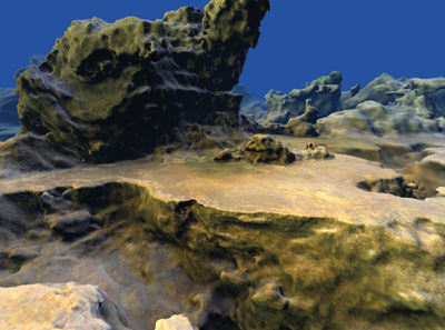
Figure 1-1 Terrain Created Entirely on the GPU
1.2 Marching Cubes and the Density Function
Conceptually, the terrain surface can be completely described by a single function, called the density function. For any point in 3D space (x, y, z), the function produces a single floating-point value. These values vary over space—sometimes positive, sometimes negative. If the value is positive, then that point in space is inside the solid terrain.
If the value is negative, then that point is located in empty space (such as air or water). The boundary between positive and negative values—where the density value is zero—is the surface of the terrain. It is along this surface that we wish to construct a polygonal mesh.
We use the GPU to generate polygons for a "block" of terrain at a time, but we further subdivide the block into 32x32x32 smaller cells, or voxels. Figure 1-2 illustrates the coordinate system. It is within these voxels that we will construct polygons (triangles) that represent the terrain surface. The marching cubes algorithm allows us to generate the correct polygons within a single voxel, given, as input, the density value at its eight corners. As output, it will produce anywhere from zero to five polygons. If the densities at the eight corners of a cell all have the same sign, then the cell is entirely inside or outside the terrain, so no polygons are output. In all other cases, the cell lies on the boundary between rock and air, and anywhere from one to five polygons will be generated.
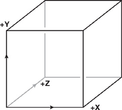
Figure 1-2 The Coordinate System Used for Voxel Space
1.2.1 Generating Polygons Within a Cell
The generation of polygons within a cell works as follows: As shown in Figure 1-3, we take the density values at the eight corners and determine whether each value is positive or negative. From each one we make a bit. If the density is negative, we set the bit to zero; if the density is positive, we set the bit to one.
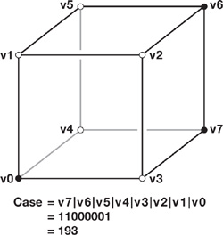
Figure 1-3 A Single Voxel with Known Density Values at Its Eight Corners
We then logically concatenate (with a bitwise OR operation) these eight bits to produce a byte—also called the case—in the range 0–255. If the case is 0 or 255, then the cell is entirely inside or outside the terrain and, as previously described, no polygons will be generated. However, if the case is in the range [1..254], some number of polygons will be generated.
If the case is not 0 or 255, it is used to index into various lookup tables (on the GPU, constant buffers are used) to determine how many polygons to output for that case, as well as how to build them. Each polygon is created by connecting three points (vertices) that lie somewhere on the 12 edges of the cell. Figure 1-4 illustrates the basic cases resulting from application of the marching cubes algorithm.
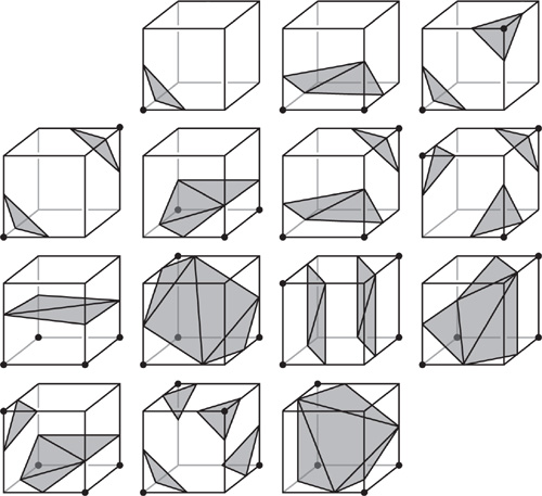
Figure 1-4 The 14 Fundamental Cases for Marching Cubes
Exactly where a vertex is placed along an edge is determined by interpolation. The vertex should be placed where the density value is approximately zero. For example, if the density at end A of the edge is 0.1 and at end B is -0.3, the vertex would be placed 25 percent of the way from A to B.
Figure 1-5 illustrates one case. After the case is used to index into lookup tables, the blue dots indicate which edges must have vertices placed on them. Gray areas show how these vertices will be connected to make triangles. Note that where the blue dots actually appear along the edges depends on the density values at the ends of the edge.
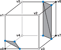
Figure 1-5 Implicit Surface to Polygon Conversion
Our output is a triangle list, so every three vertices that are output create a triangle, and the next vertex output begins a new triangle. If a certain case requires that we generate N polygons, we will need to generate a vertex (somewhere along one of the cell's edges) 3xN times.
1.2.2 Lookup Tables
Two primary lookup tables are at work here. The first, when indexed by the case number, tells us how many polygons to create for that case:
int case_to_numpolys[256];The second lookup table is much larger. Once it receives the case number, the table provides the information needed to build up to five triangles within the cell. Each of the five triangles is described by just an int3 value (three integers); the three values are the edge numbers [0..11] on the cube that must be connected in order to build the triangle. Figure 1-6 shows the edge-numbering scheme.
int3 edge_connect_list[256][5];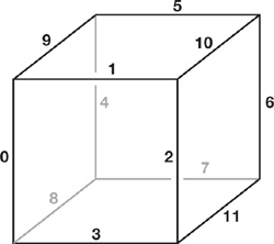
Figure 1-6 The Edge Numbers Assigned to the 12 Edges of a Voxel
For example, if the case number is 193, then looking up case_to_numpolys[193] would tell us how many polygons we need to generate, which is 3. Next, the edge_connect_list[193][] lookups would return the following values:
int3 edge_connect_list[193][0] : 11 5 10
int3 edge_connect_list[193][1] : 11 7 5
int3 edge_connect_list[193][2] : 8 3 0
int3 edge_connect_list[193][3] : -1 -1 -1
int3 edge_connect_list[193][4] : -1 -1 -1
To build the triangles within this cell, a geometry shader would generate and stream out nine vertices (at the appropriate places along the edges listed)—forming three triangles—to a vertex buffer for storage. Note that the last two int3 values are -1; these values will never even be sampled, though, because we know there are only three triangles for this case. The GPU would then move on to the next cell.
We encourage you to copy the lookup tables from the demo on this book's accompanying DVD, because generating the tables from scratch can be time-consuming. The tables can be found in the file models\tables.nma.
1.3 An Overview of the Terrain Generation System
We divide the world into an infinite number of equally sized cubic blocks, as already described. In the world-space coordinate system, each block is 1x1x1 in size. However, within each block are 323 voxels that potentially contain polygons. A pool of around 300 vertex buffers are dynamically assigned to the blocks currently visible in the view frustum, with higher priority given to the closest blocks. As new blocks come into the view frustum (as the user moves around), the farthest away or newly view-cullable vertex buffers are evicted and reused for the newly wished-for blocks.
Not all blocks contain polygons. Whether they do or not depends on complex calculations, so usually we won't know if they contain polygons until we try to generate the blocks. As each block is generated, a stream-out query asks the GPU if any polygons were actually created. Blocks that don't produce polygons—this is common—are flagged as "empty" and put into a list so they won't be uselessly regenerated. This move also prevents those empty blocks from unnecessarily occupying a vertex buffer.
For each frame, we sort all the vertex buffers (their bounding boxes are well known) from front to back. We then generate any new blocks that are needed, evicting the most distant block whenever we need a free vertex buffer. Finally, we render the sorted blocks from front to back so that the GPU doesn't waste time shading pixels that might be occluded by other parts of the terrain.
1.3.1 Generating the Polygons Within a Block of Terrain
Conceptually, generating a block of terrain involves two main steps. We outline the steps here and then elaborate upon them in the following subsections.
- First, we use the GPU's pixel shader (PS) unit to evaluate the complex density function at every cell corner within the block and store the results in a large 3D texture. The blocks are generated one at a time, so one 3D texture can be shared universally. However, because the texture stores the density values at the cell corners, the texture is 33x33x33 in size, rather than 32x32x32 (the number of cells in the block).
- Next, we visit each voxel and generate actual polygons within it, if necessary. The polygons are streamed out to a vertex buffer, where they can be kept and repeatedly rendered to the screen until they are no longer visible.
1.3.2 Generating the Density Values
Rendering to a 3D texture is a somewhat new idea, and it's worthy of some explanation here. On the GPU, a 3D texture is implemented as an array of 2D textures. To run a PS that writes to every pixel in a slice, we draw two triangles that, together, cover the render portal. To cover all the slices, we use instancing. In DirectX, this means nothing more than calling ID3D10Device::DrawInstanced() (rather than the ordinary Draw() function) with the numInstances parameter set to 33. This procedure effectively draws the triangle pair 33 times.
The vertex shader (VS) knows which instance is being drawn by specifying an input attribute using the SV_InstanceID semantic; these values will range from 0 to 32, depending on which instance is being drawn. The VS can then pass this value on to the geometry shader, which writes it out to an attribute with the SV_RenderTarget - ArrayIndex semantic. This semantic determines to which slice of the 3D texture (the render target array) the triangle actually gets rasterized. In this way, the PS is run on every pixel in the entire 3D texture. On the book's DVD, see shaders\1b_build_density_vol.vsh and .gsh.
Conceptually, the PS that shades these triangles takes, as input, a world-space coordinate and writes, as output, a single, floating-point density value. The math that converts the input into the output is our density function.
1.3.3 Making an Interesting Density Function
The sole input to the density function is this:
float3 ws;This value is the world-space coordinate. Luckily, shaders give us plenty of useful tools to translate this value into an interesting density value. Some of the tools at our disposal include the following:
- Sampling from source textures, such as 1D, 2D, 3D, and cube maps
- Constant buffers, such as lookup tables
- Mathematical functions, such as cos(), sin(), pow(), exp(), frac(), floor(), and arithmetic
For example, a good starting point is to place a ground plane at y = 0:
float density = -ws.y;This divides the world into positive values, those below the y = 0 plane (let's call that earth), and negative values, those above the plane (which we'll call air). A good start! Figure 1-7 shows the result.
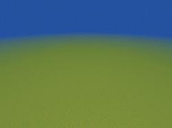
Figure 1-7 We Start with a Flat Surface
Next, let's make the ground more interesting by adding a bit of randomness, as shown in Figure 1-8. We simply use the world-space coordinate (ws) to sample from a small (163) repeating 3D texture full of random ("noise") values in the range [-1..1], as follows:
density += noiseVol.Sample(TrilinearRepeat, ws).x;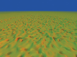
Figure 1-8 Terrain with One Level of Noise
Figure 1-8 shows how the ground plane warps when a single octave of noise is added.
Note that we can scale ws prior to the texture lookup to change the frequency (how quickly the noise varies over space). We can also scale the result of the lookup before adding it to the density value; scaling changes the amplitude, or strength, of the noise. To generate the image in Figure 1-9, the following line of shader code uses a noise "function" with twice the frequency and half the amplitude of the previous example:
density += noiseVol.Sample(TrilinearRepeat, ws * 2).x * 0.5;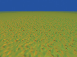
Figure 1-9 One Octave of Noise with Twice the Frequency but Half the Amplitude of
One octave (sample) of noise isn't that interesting; using three octaves is an improvement, as Figure 1-10 shows. To be optimal, the amplitude of each octave should be half that of the previous octave, and the frequency should be roughly double the frequency of the previous octave. It's important not to make the frequency exactly double, though. The interference of two overlapping, repeating signals at slightly different frequencies is beneficial here because it helps break up repetition. Note that we also use three different noise volumes.
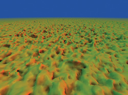
Figure 1-10 Three Octaves at High Frequency Generate More Details
density += noiseVol1.Sample(TrilinearRepeat, ws * 4.03).x * 0.25;
density += noiseVol2.Sample(TrilinearRepeat, ws * 1.96).x * 0.50;
density += noiseVol3.Sample(TrilinearRepeat, ws * 1.01).x * 1.00;
If more octaves of noise are added at progressively lower frequencies (and higher amplitudes), larger terrain structures begin to emerge, such as large mountains and trenches. In practice, we need about nine octaves of noise to create a world that is rich in both of these low-frequency features (such as mountains and canyons), but that also retains interesting high-frequency features (random detail visible at close range). See Figure 1-11.
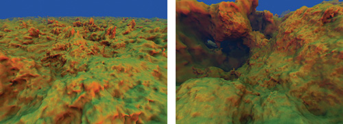
Figure 1-11 Adding Lower Frequencies at Higher Amplitude Creates Mountains
Sampling Tips
It's worth going over a few details concerning sampling the various octaves. First, the world-space coordinate can be used, without modification, to sample the seven or eight highest-frequency octaves. However, for the lowest octave or two, the world-space coordinate should first be slightly rotated (by 3x3 rotation matrices) to reduce repetition of the most salient features of the terrain. It's also wise to reuse three or four noise textures among your nine octaves to improve cache coherency; this reuse will not be noticeable at significantly different scales.
Finally, precision can begin to break down when we sample extremely low frequency octaves of noise. Error begins to show up as (unwanted) high-frequency noise. To work around this, we manually implement trilinear interpolation when sampling the very lowest octave or two, using full floating-point precision. For more information on how to do this, see the comments and code in shaders\density.h.
Using many octaves of noise creates detail that is isotropic (equal in all directions), which sometimes looks a bit too regular. One way to break up this homogeneity is to warp the world-space coordinate by another (low-frequency) noise lookup, before using the coordinate for the nine noise lookups. At a medium frequency and mild amplitude, the warp creates a surreal, ropey, organic-looking terrain, as shown in Figure 1-12. At a lower frequency and higher amplitude, the warp can increase the occurrence of caves, tunnels, and arches. The effects can easily be combined, of course, by summing two octaves.
// Do this before using 'ws' to sample the nine octaves!
float3 warp = noiseVol2.Sample( TrilinearRepeat, ws*0.004 ).xyz;
ws += warp * 8;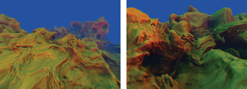
Figure 1-12 Warping the World-Space Coordinate Creates a Surreal-Looking Terrain
We can also introduce a hard "floor" to the scene by very suddenly boosting the density values below a certain y coordinate. To some degree, this mimics sediment deposition in nature, as eroded sediment finds its way to lower areas and fills them in. Visually, it makes the scene feel less aquatic and more landlike, as shown in Figure 1-13.
float hard_floor_y = -13;
density += saturate((hard_floor_y - ws_orig.y) * 3) * 40;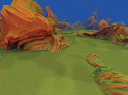
Figure 1-13 A Floor Level Can Be Introduced
Many other interesting effects can be accomplished by adjusting only the density value by the world-space y coordinate. We can make the adjustment by using either the prewarp or the post-warp world-space coordinate. If we use the post-warp, then under its influence any effects that look like shelves or terraces will appear to melt and sag, along with the rest of the terrain. Figures 1-14 and 1-15 show two examples.
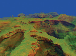
Figure 1-14 Building Shelves
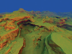
Figure 1-15 Repeating Terraces
These are very basic techniques. Myriad effects are possible, of course, and can be easily prototyped by modifying shaders\density.h.
1.3.4 Customizing the Terrain
All of the techniques we have discussed so far contribute to producing a nice, organic-looking terrain. However, for practical use, we must be able to domesticate the shape of the terrain. There are many ways to do this.
Use a Hand-Painted 2D Texture
Stretch a hand-painted 2D texture over a very large area (one that would take, say, 10 minutes to "walk across" in your demo or game). The density function could sample this 2D texture using ws.xz and use the result to drive the eight noise lookups. The red channel of the texture could influence the scaling of ws.y before using it for the lookups, resulting in the noise appearing vertically squished in some areas or stretched in others. The green channel could modulate the amplitudes of the higher-frequency octaves of noise, causing the terrain to look rocky in some places and smoother in others. And the blue channel could even modulate the warp effect discussed earlier, so that some areas look more "alien" than others.
Add Manually Controlled Influences
It's also possible to add manually controlled influences to the density field. So, if your game level needs a flat spot for a ship to land, as in Figure 1-16, you could pass data to describe it to the pixel shader in a constant buffer. The shader code might then look something like the following:
float distance_from_flat_spot = length(ws.xz – flat_spot_xz_coord);
float flatten_amount = saturate(outer_radius – distance_from_flat_spot)/
        (outer_radius – inner_radius) ) * 0.9;
density = lerp(density, ws.y – flat_spot_height, flatten_amount);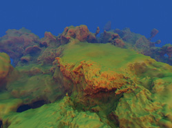
Figure 1-16 This "Man-Made" Flat Spot Creates an Ideal Landing Place for Aircraft
Here, the density function will be 90 percent replaced by the "flat spot" function within inner_radius world-space units of its center; however, by a distance of outer_radius, the influence drops off to zero (saturate() clamps a value to the 0..1 range). In addition, many flat spots could be used across your terrain—at varying heights, weights, and radii of influence. These flat spots are obtained for the cost of just one flat spot, as long as there is enough distance between them that an individual block of terrain will only be affected by, at most, one flat spot at a time. (Of course, dynamic looping could also be used if you need more than one per block.) The application is responsible for updating the constant buffer with the relevant information whenever a block is to be generated.
Add Miscellaneous Effects
Other effects are possible by combining all the previous techniques—from caves, to cliffs, to painted maps of rivers. If you can imagine it, you can probably code it. Want a spherical planet, as in Figure 1-17? Instead of using the y plane as a ground, try this (plus noise):
float rad = 80;
float density = rad - length(ws – float3(0, -rad, 0));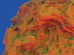
Figure 1-17 A Spherical Planet
Or, for a never-ending 3D network of caves, try this (plus noise):
// This positive starting bias gives us a little more rock than open space.
float density = 12;
The density function used in the demo can be modified by editing shaders\density.h, which is included by several other shaders in the demo. If you'd like to make changes in real time, do this: Run the demo in windowed mode (see bin\args.txt), edit the density function to your liking, and then press F9 (Reload Shaders) followed by "Z" (Regenerate Terrain).
1.4 Generating the Polygons Within a Block of Terrain
There are many ways to break up the task of generating a block of terrain on the GPU. In the simplest approach, we generate density values throughout a 3D texture (representing the corners of all the voxels in the block) in one render pass. We then run a second render pass, where we visit every voxel in the density volume and use the GS to generate (and stream out to a vertex buffer) anywhere from 0 to 15 vertices in each voxel. The vertices will be interpreted as a triangle list, so every 3 vertices make a triangle.
For now, let's focus on what we need to do to generate just one of the vertices. There are several pieces of data we'd like to know and store for each vertex:
- The world-space coordinate
- The world-space normal vector (used for lighting)
- An "ambient occlusion" lighting value
These data can be easily represented by the seven floats in the following layout. Note that the ambient occlusion lighting value is packed into the .w channel of the first float4.
struct rock_vertex
{
  float4 wsCoordAmbo;
  float3 wsNormal;
};
The normal can be computed easily, by taking the gradient of the density function (the partial derivative, or independent rate of change, in the x, y, and z directions) and then normalizing the resulting vector. This is easily accomplished by sampling the density volume six times. To determine the rate of change in x, we sample the density volume at the next texel in the +x direction, then again at the next texel in the -x direction, and take the difference; this is the rate of change in x. We repeat this calculation in the y and z directions, for a total of six samples. The three results are put together in a float3, and then normalized, producing a very high quality surface normal that can later be used for lighting. Listing 1-1 shows the shader code.
Example 1-1. Computing the Normal via a Gradient
float d = 1.0 / (float)voxels_per_block;
float3 grad;
grad.x = density_vol.Sample(TrilinearClamp, uvw + float3(d, 0, 0)) -
         density_vol.Sample(TrilinearClamp, uvw + float3(-d, 0, 0));
grad.y = density_vol.Sample(TrilinearClamp, uvw + float3(0, d, 0)) -
         density_vol.Sample(TrilinearClamp, uvw + float3(0, -d, 0));
grad.z = density_vol.Sample(TrilinearClamp, uvw + float3(0, 0, d)) -
         density_vol.Sample(TrilinearClamp, uvw + float3(0, 0, -d));
output.wsNormal = -normalize(grad);
The ambient occlusion lighting value represents how much light, in general, is likely to reach the vertex, based on the surrounding geometry. This value is responsible for darkening the vertices that lie deep within nooks, crannies, and trenches, where less light would be able to penetrate. Conceptually, we could generate this value by first placing a large, uniform sphere of ambient light that shines on the vertex. Then we trace rays inward to see what fraction of the vertices could actually reach the vertex without colliding with other parts of the terrain, or we could think of it as casting many rays out from the vertex and tracking the fraction of rays that can get to a certain distance without penetrating the terrain. The latter variant is the method our terrain demo uses.
To compute an ambient occlusion value for a point in space, we cast out 32 rays. A constant Poisson distribution of points on the surface of a sphere works well for this. We store these points in a constant buffer. We can—and should—reuse the same set of rays over and over for each vertex for which we want ambient occlusion. (Note: You can use our Poisson distribution instead of generating your own; search for "g_ray_dirs_32" in models\tables.nma on the book's DVD.) For each of the rays cast, we take 16 samples of the density value along the ray—again, just by sampling the density volume. If any of those samples yields a positive value, the ray has hit the terrain and we consider the ray fully blocked. Once all 32 rays are cast, the fraction of them that were blocked—usually from 0.5 to 1—becomes the ambient occlusion value. (Few vertices have ambient occlusion values less than 0.5, because most rays traveling in the hemisphere toward the terrain will quickly be occluded.)
Later, when the rock is drawn, the lighting will be computed as usual, but the final light amount (diffuse and specular) will be modulated based on this value before we apply it to the surface color. We recommend multiplying the light by saturate(1 – 2*ambient_occlusion), which translates an occlusion value of 0.5 into a light multiplier of 1, and an occlusion value of 1 to a light multiplier of 0. The multiplier can also be run through a pow() function to artistically influence the falloff rate.
1.4.1 Margin Data
You might notice, at this point, that some of the occlusion-testing rays go outside the current block of known density values, yielding bad information. This scenario would create lighting artifacts where two blocks meet. However, this is easily solved by enlarging our density volume slightly and using the extra space to generate density values a bit beyond the borders of our block. The block might be divided into 323 voxels for tessellation, but we might generate density values for, say, a 443 density volume, where the extra "margin" voxels represent density values that are actually physically outside of our 323 block. Now we can cast occlusion rays a little farther through our density volume and get more-accurate results. The results still might not be perfect, but in practice, this ratio (32 voxels versus 6 voxels of margin data at each edge) produces nice results without noticeable lighting artifacts. Keep in mind that these dimensions represent the number of voxels in a block; the density volume (which corresponds to the voxel corners) will contain one more element in each dimension.
Unfortunately, casting such short rays fails to respect large, low-frequency terrain features, such as the darkening that should happen inside large gorges or holes. To account for these low-frequency features, we also take a few samples of the real density function along each ray, but at a longer range—intentionally outside the current block. Sampling the real density function is much more computationally expensive, but fortunately, we need to perform sampling only about four times for each ray to get good results. To lighten some of the processing load, we can also use a "lightweight" version of the density function. This version ignores the higher-frequency octaves of noise because they don't matter so much across large ranges. In practice, with eight octaves of noise, it's safe to ignore the three highest-frequency octaves.
The block of pseudocode shown in Listing 1-2 illustrates how to generate ambient occlusion for a vertex.
Note the use of saturate(d * 9999), which lets any positive sample, even a tiny one, completely block the ray. However, values deep within the terrain tend to have progressively higher density values, and values farther from the terrain surface do tend to progressively become more negative. Although the density function is not strictly a signed distance function, it often resembles one, and we take advantage of that here.
Example 1-2. Pseudocode for Generating Ambient Occlusion for a Vertex
float visibility = 0;
for (ray = 0 ..31)
{
  float3 dir = ray_dir[ray];
  // From constant buffer
  float this_ray_visibility = 1;
  // Short-range samples from density volume:
  for (step = 1 ..16)
  // Don't start at zero
  {
    float d = density_vol.Sample(ws + dir * step);
    this_ray_visibility *= saturate(d * 9999);
  }
  // Long-range samples from density function:
  for (step = 1 ..4)
  // Don't start at zero!
  {
    float d = density_function(ws + dir * big_step);
    this_ray_visibility *= saturate(d * 9999);
  }
  visibility += this_ray_visibility;
}
return (1 – visibility / 32.0); // Returns occlusion
During ray casting, instead of strictly interpreting each sample as black or white (hit or miss), we allow things to get "fuzzy." A partial occlusion happens when the sample is near the surface (or not too deep into the surface). In the demo on the book's DVD, we use a multiplier of 8 (rather than 9999) for short-range samples, and we use 0.5 for long-range samples. (Note that these values are relative to the range of values that are output by your particular density function). These lower multipliers are especially beneficial for the long-range samples; it becomes difficult to tell that there are only four samples being taken. Figures 1-18 through 1-20 show some examples.
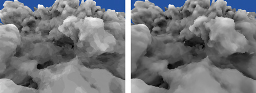
Figure 1-18 Long-Range Ambient Occlusion Only
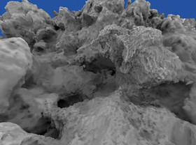
Figure 1-19 Both Long-Range and Short-Range Ambient Occlusion
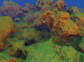
Figure 1-20 The Regular Scene, Shaded Using Ambient Occlusion
1.4.2 Generating a Block: Method 1
This section outlines three methods for building a block. As we progress from method 1 to method 3, the techniques get successively more complex, but faster.
The first (and simplest) method for building a block of terrain is the most straight forward, and requires only two render passes, as shown in Table 1-1.
Table 1-1. Method 1 for Generating a Block
|
Pass Name |
Description |
Geometry Shader Output Struct |
|
build_densities |
Fill density volume with density values. |
N/A |
|
gen_vertices |
Visit each (nonmargin) voxel in the density volume. The geometry shader generates and streams out up to 15 vertices (5 triangles) per voxel. |
Count: 0/3/6/9/12/15 |
However, this method is easily optimized. First, the execution speed of a geometry shader tends to decrease as the maximum size of its output (per input primitive) increases. Here, our maximum output is 15 vertices, each consisting of 7 floats—for a whopping 105 floats. If we could reduce the floats to 32 or less—or even 16 or less—the GS would run a lot faster.
Another factor to consider is that a GS is not as fast as a VS because of the geometry shader's increased flexibility and stream-out capability. Moving most of the vertex generation work, especially the ambient occlusion ray casting, into a vertex shader would be worthwhile. Fortunately, we can accomplish this, and reduce our GS output size, by introducing an extra render pass.
1.4.3 Generating a Block: Method 2
The problems described in method 1—extremely large geometry shader output (per input primitive) and the need to migrate work from the geometry shaders to the vertex shaders—are resolved by this design, shown in Table 1-2, which is an impressive 22 times faster than method 1.
Table 1-2. Method 2 for Generating a Block
|
Pass Name |
Description |
Geometry Shader Output Struct |
|
build_densities |
Fill density volume with density values. |
N/A |
|
list_triangles |
Visit each voxel in the density volume; stream out a lightweight marker point for each triangle to be generated. Use a stream-out query to skip remaining passes if no output here. |
uint z6_y6_x6_edge1_edge2_edge3; Count: 0–5 |
|
gen_vertices |
March through the triangle list, using the vertex shader to do most of the work for generating the vertex. The geometry shader is a pass-through, merely streaming the result out to a buffer. |
Count: 3 |
Here, the gen_vertices pass has been broken into list_triangles and gen_vertices. The list_triangles pass has much smaller maximum output; it outputs, at most, five marker points. Each point represents a triangle that will be fleshed out later, but for now, it's only a single uint in size (an unsigned integer—the same size as a float). Our maximum output size has gone from 105 to 5, so the geometry shader will execute much faster now.
The crucial data for generating each triangle is packed into the uint:
struct triangle_marker_point
{
uint z6_y6_x6_edge1_edge2_edge3;
};Six integer values are packed into this one uint, which tells us everything we need to build a triangle within this voxel. The x, y, and z bit fields (6 bits each, or [0..31]) indicate which voxel, within the current block, should contain the generated triangle. And the three edge fields (each 4 bits) indicate the edge [0..11] along which the vertex should be placed. This information, plus access to the density volume, is all the vertex shader in the last pass needs to generate the three vertices that make up the triangle. In that final pass, all three vertices are generated in a single execution of the vertex shader and then passed to the geometry shader together, in a large structure, like this:
struct v2gConnector
{
float4 wsCoordAmbo1;
float3 wsNormal1;
float4 wsCoordAmbo2;
float3 wsNormal2;
float4 wsCoordAmbo3;
float3 wsNormal3;
};The GS then writes out three separate vertices from this one big structure. This activity produces a triangle list identical to what method 1 produced, but much more quickly.
Adding another render pass is helpful because it lets us skip the final (and most expensive) pass if we find that there are no triangles in the block. The test to determine if any triangles were generated merely involves surrounding the list_triangles pass with a stream output query (ID3D10Query with D3D10_QUERY_SO_STATISTICS), which returns the number of primitives streamed out. This is another reason why we see such a huge speed boost between methods 1 and 2.
Method 2 is faster and introduces the useful concept of adding a new render pass to migrate heavy GS work into the VS. However, method 2 has one major flaw: it generates each final vertex once for each triangle that uses it. A vertex is usually shared by an average of about five triangles, so we're doing five times more work than we need to.
1.4.4 Generating a Block: Method 3
This method generates each vertex once, rather than an average of five times, as in the previous methods. Despite having more render passes, method 3 is still about 80 percent faster than method 2. Method 3, instead of producing a simple, nonindexed triangle list in the form of many vertices (many of them redundant), creates a vertex pool and a separate index list. The indices in the list are now references to the vertices in the vertex pool, and every three indices denote a triangle.
To produce each vertex only once, we limit vertex production within a cell to only edges 3, 0, and 8. A vertex on any other edge will be produced by another cell—the one in which the vertex, conveniently, does fall on edge 3, 0, or 8. This successfully produces all the needed vertices, just once.
Within a cell, knowing whether a vertex is needed along a particular edge (3, 0, or 8) is as simple as checking if the case number bits are different at the two corners that the edge connects. See shaders\4_list_vertices_to_generate.vsh for an example of how to do this, but note that it could also be done easily using a lookup table.
The render passes to generate vertices uniquely are shown in Table 1-3.
Table 1-3. Method 3 for Generating a Block
|
Pass Name |
Description |
Geometry Shader Output Struct |
|
build_densities |
Fill density volume with density values. |
N/A |
|
list_nonempty_cells |
Visit each voxel in the density volume; stream out a lightweight marker point for each voxel that needs triangles in it. Use a stream-out query to skip remaining passes if no output here. |
uint z8_y8_x8_case8; Count: 0–1 Note: Includes an extra row of voxels at the far end of x, y, and z. |
|
list_verts_to_generate |
Marches nonempty_cell_list and looks only at edges 3, 0, and 8; streams out a marker point for each one that needs a vertex on it. |
uint z8_y8_x8_null4_edge4; Count: 0–3 |
|
gen_vertices |
Marches vert_list and generates the final (real) vertices. VS does the bulk of the work to generate the real vertex; GS just streams it out. |
float4 wsCoordAmbo;
float3 wsNormal;
Count: 1 |
The previous passes generate our vertices without redundancy, but we still need to generate our index list. This is the most difficult concept in method 3. To make it work, we'll need a temporary volume texture, VertexIDVol. This is a 323 volume texture of the format DXGI_FORMAT_R32_UINT, so each voxel can hold a single uint.
The problem is that when generating the indices for a given (nonempty) cell, we have no idea where the indices are in the vertex buffer, that magical storage structure where all those streamed-out vertices have been consolidated for us. (Remember, only a small fraction of cells actually generate vertices.) The 3D texture is our solution; we use it to splat the vertex ID (or index within the vertex buffer) of each vertex into a structure that we can look up into randomly. Sampling this volume can then act as a function that takes, as input, a 3D location (within the block) and provides, as output, the vertex ID (or index in the vertex buffer) of the vertex that was generated there. This is the missing information we need to be able to generate an index list to connect our vertices into triangles. The two extra render passes are described in Table 1-4.
Table 1-4. Method 3 for Generating the Index Buffer
|
Pass Name |
Description |
Geometry Shader Output Struct |
|
splat_vertex_ids |
Marches vert_list and splats each one's SV_VertexID to VertexIDVol. |
(No stream output; pixel shader just writes out SV_VertexID.) |
|
gen_indices |
Marches nonempty_cell_list and streams out up to 15 uints per cell—the indices to make up to five triangles. Samples VertexIDVol to get this information. |
uint index; Count: 15 Note: Do not output any indices for cells in any final row (in x/y/z). |
The splat is accomplished by drawing a single point into a voxel of the 3D texture. The xy coordinates are taken from the block-space xy coordinate, and using the block-space z coordinate, the GS routes the point to the correct slice in the 3D texture. The value written out in the PS is the value that came into the VS as SV_VertexID, which is a system-generated value indicating the zero-based index of the vertex in our vert_list vertex buffer. Note that it's not necessary to clear the VertexIDVol prior to splatting.
When sampling the volume to fetch a vertex ID, note that if you need the vertex ID for a vertex on an edge other than 3, 0, or 8, you will instead have to sample the appropriate neighbor voxel along edge 3, 0, or 8. The mechanics for this actually turn out to be trivial; see shaders\7_gen_indices.gsh on the DVD.
You might notice that we would often be splatting up to three vertices per voxel, but we're only writing to a one-channel texture! Thus, if a single cell had vertices on edges 3 and 8, the VertexIDVol could hold the index for only one of them. The easy solution is to triple the width of the vertex ID volume (making it 3NxNxN in size). When splatting, multiply the integer block-space x coordinate by 3, then add 0, 1, or 2 depending on which edge you're splatting the vertex ID for (3, 0, or 8, respectively). (See shaders\5b_splat_vertex_IDs.vsh.) In the final pass, when you're sampling the results, adjust the x coordinate similarly, depending whether you want the vertex ID along edge 3, 0, or 8 within that voxel. (See shaders\7_gen_indices.gsh.)
Also note that in method 3, the list_nonempty_cells pass includes an extra layer of cells at the far ends of the x, y, and z axes. Sometimes vertices will be needed that fall on an edge other than 3, 0, or 8 in the final row of cells, so this ensures that the vertices are all created—even if the cell in which they do map onto edge 3, 0, or 8 happens to be in a neighboring block. In the gen_indices pass, which operates on nonempty_cell_list, index generation is skipped for cells that are actually beyond the current block. (See shaders\7_gen_indices.gsh for an example.)
Method 3 allows us to share vertices and, as a result, generate about one-fifth as many of them. This is quite a savings, considering that each vertex samples the complex density function 128 times (32 rays x 4 long-range occlusion samples per ray).
Using the density function and settings that ship with the demo for this chapter, an NVIDIA GeForce 8800 GPU can generate about 6.6 blocks per second using method 1, about 144 blocks per second using method 2, and about 260 blocks per second using method 3.
1.5 Texturing and Shading
One challenge with procedural generation of terrains, or any shape of arbitrary topology, is texturing—specifically, generating texture coordinates, commonly known as UVs. How can we seamlessly map textures onto these polygons with minimal distortion? A single planar projection, like the one shown in Figure 1-21, of a seamless and repeating 2D texture looks good from one angle, but inferior from others, because of intense stretching (see also Figure 1-23).
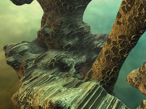
Figure 1-21 A Single Planar Projection Is Plagued by Distortion
A simple way to resolve this is to use triplanar texturing, or three different planar projections, one along each of the three primary axes (x, y, and z). At any given point, we use the projection that offers the least distortion (stretching) at that point—with some projections blending in the in-between areas, as in Figure 1-22. For example, a surface point whose normal vector pointed mostly in the +x or -x direction would use the yz planar projection. A blending range of roughly 10 to 20 degrees tends to work well; see Figure 1-23 for an illustration of how wide the blending range is.
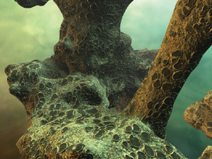
Figure 1-22 Three Planar Projections of the Same Texture, Blended Together Based on the Surface Normal Vector
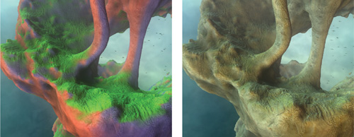
Figure 1-23 Triplanar Texturing
When we use bump mapping with triplanar texturing, we need to make sure the tangent basis is generated from the normal separately for each projection. For example, for the x-projection, a very crude world-space tangent basis could simply be the vectors <0, 1, 0> and <0, 0, 1>. However, we can do much better than this. Fortunately, it is very easy to generate the real tangent basis from the normal. Here, 90-degree rotations of vectors amount to just swizzling two of the components and flipping the sign on one of them. For example, for the x-projection, you might use the vectors <normal.z, normal.y, -normal.x> and <normal.y, -normal.x, normal.z>. However, note that the location of the negative sign depends on the way the data is stored in the bump maps.
Triplanar texturing can be done in a single render pass, as shown in the pixel shader code sample in Listing 1-3. The sample fetches the color values and bump vectors for each of the three planar projections and then blends them together based on the normal. Finally, the blended bump vector is applied to the vertex-interpolated normal to yield a bumped normal.
Another convenient way to texture the terrain is by mapping certain height values to certain colors, creating striations. With graphics hardware, this translates into a 1D texture lookup that uses the world-space y coordinate—or, better, use a 2D texture lookup. In the texture, let the color scheme vary across the u axis, and let the v axis represent the altitude. When doing the lookup, use a single octave of very low frequency noise to drive the u coordinate, so that the color scheme changes as the viewer roams.
Example 1-3. Texture Planar Projection
// Determine the blend weights for the 3 planar projections.
        // N_orig is the vertex-interpolated normal vector.
        float3 blend_weights = abs( N_orig.xyz );
// Tighten up the blending zone:
        blend_weights = (blend_weights - 0.2) * 7;
        blend_weights = max(blend_weights, 0); Force weights to sum to 1.0 (very important!)
        blend_weights /= (blend_weights.x + blend_weights.y + blend_weights.z ).xxx;
        // Now determine a color value and bump vector for each of the 3projections, blend them, and store blended results in these two vectors:
        float4 blended_color; // .w hold spec value
        float3 blended_bump_vec;
{
  // Compute the UV coords for each of the 3 planar
  // projections. // tex_scale (default ~ 1.0) determines how big the textures
  // appear.
  float2 coord1 = v2f.wsCoord.yz * tex_scale;
  float2 coord2 = v2f.wsCoord.zx * tex_scale;
  float2 coord3 = v2f.wsCoord.xy * tex_scale; //
  // This is where you would apply conditional displacement mapping.
  // if (blend_weights.x > 0) coord1 = . . .
  // if (blend_weights.y > 0)coord2 =...
  // if (blend_weights.z > 0) coord3 = . . .
  // Sample color maps for
  // each projection, at those UV coords.
  float4 col1 = colorTex1.Sample(coord1);
  float4 col2 = colorTex2.Sample(coord2);
  float4 col3 = colorTex3.Sample(coord3);
  // Sample bump maps too, and generate bump vectors.
  // (Note: this uses an oversimplified tangent basis.)
  float2 bumpFetch1 = bumpTex1.Sample(coord1).xy - 0.5;
  float2 bumpFetch2 = bumpTex2.Sample(coord2).xy - 0.5;
  float2 bumpFetch3 = bumpTex3.Sample(coord3).xy - 0.5;
  float3 bump1 = float3(0, bumpFetch1.x, bumpFetch1.y);
  float3 bump2 = float3(bumpFetch2.y, 0, bumpFetch2.x);
  float3 bump3 = float3(bumpFetch3.x, bumpFetch3.y, 0);
  // Finally, blend the results of the 3 planar projections.
  blended_color = col1.xyzw * blend_weights.xxxx +
                  col2.xyzw * blend_weights.yyyy +
                  col3.xyzw * blend_weights.zzzz;
  blended_bump_vec = bump1.xyz * blend_weights.xxx +
                     bump2.xyz * blend_weights.yyy +
                     bump3.xyz * blend_weights.zzz;
}
// Apply bump vector to vertex-interpolated normal vector.
float3 N_for_lighting = normalize(N_orig + blended_bump);
To make it even more interesting, make the low-frequency noise vary slowly on x and z but quickly on y—this approach will make the color scheme vary with altitude, as well. It's also fun to add a small amount of the normal vector's y component to the u coordinate for the lookup; this helps break up the horizontal nature of the striations. Figures 1-24 and 1-25 illustrate these techniques.
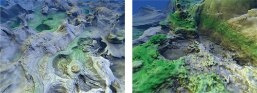
Figure 1-24 The Striation Technique

Figure 1-25 The Variable Climate Lookup Texture
Planar 2D projections and altitude-based lookups are very useful for projecting detailed, high-resolution 2D textures onto terrain. However, texturing can also be done procedurally. For example, a few octaves of noise—based on the world-space coordinate—can be used to perturb the normal vector, adding a few extra octaves of perceived detail, as shown in Listing 1-4 and Figure 1-26.
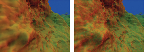
Figure 1-26 Textured Terrain
Example 1-4. Normal Vector Perturbation
// Further perturb normal vector by a few octaves of procedural noise.
        float3 v = 0;
        v += noiseVol1.Sample(ws* 3.97)*1.00;
        v += noiseVol2.Sample(ws* 8.06)*0.50;
        v += noiseVol3.Sample(ws*15.96)*0.25;
        N = normalize(N + v);
The base surface color can also be generated or modified procedurally. For example, a simple marble texture can be created by warping the world-space coordinate by several octaves of lower-frequency noise, then taking sin(ws.y), as shown in Listing 1-5 and Figure 1-27.
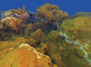
Figure 1-27 Terrain with Marble Texture
Texture projection and procedural texturing are very powerful tools that can be combined easily to achieve a large variety of effects. Used alone, procedural texturing tends to lack the high-resolution detail that a texture (such as a photograph or a painted map) can offer. On the other hand, texture projection used alone looks repetitive over a very large space. However, simple and creative combinations of both tools can solve these problems and create beautifully textured landscapes with impressive detail and variety.
Example 1-5. Marble Texture Generation
// Use warped world-space coordinate to generate a marble texture.
float3 v = 0;
v += noiseVol2.Sample(ws * 0.47) * 1.00;
v += noiseVol3.Sample(ws * 1.06) * 0.50;
v += noiseVol1.Sample(ws * 1.96) * 0.25;
float3 ws_warped = ws + v;
float is_marble = pow(saturate(sin(ws_warped.y) * 1.1), 3.0);
float3 marble_color = 1;
blended_color = lerp(blended_color, marble_color, is_marble);
1.6 Considerations for Real-World Applications
1.6.1 Level of Detail
In an ideal 3D scene, all polygons would show up at about the same size on the screen. In practice, though, this rarely happens. The terrain technique presented so far has created a tessellation that is somewhat uniform in world space, but definitely not uniform in screen space. As a result, distant polygons appear very tiny (one pixel or less in size), which is wasteful, and introduces aliasing artifacts. To alleviate this problem, we'd like to divide blocks into three groups: close, medium, and far. Blocks at close range will have polygons at a regular size, and blocks at a medium distance will have larger polygons (in world space). Finally, blocks at a far distance will have the largest polygons. To implement this approach, we can choose from two basic schemes: one in which lower-level-of-detail (LOD) blocks have fewer polygons in them, and another where lower-LOD blocks simply represent a larger space.
In the "fewer polygons" scheme, all blocks remain at 1x1x1 in world space, but faraway blocks have a smaller internal grid size (163 or 83 instead of 323). Unfortunately, this scheme causes the number of blocks to bloat very quickly, which rapidly decreases performance—for both the rendering and, especially, the generation of blocks.
The "bigger blocks" scheme is a better approach. Here, all blocks have a constant 323 internal grid size, but the world-space size of the terrain that the blocks represent changes, based on their distance from the viewer. Nearby blocks will occupy a cube that is 1x1x1 in world space, while larger blocks (for terrain that is farther away) will cover a 2x2x2 cube in world space and some even larger cubes (4x4x4) out to a great distance. At draw time, we draw the large (faraway) blocks first, then the medium blocks, then the fine blocks (1x1x1) overtop. Because the number of blocks remains manageable, this is the preferred scheme.
As with many LOD schemes, however, switching a section of terrain from one LOD to another creates a sudden, visual popping artifact. The easiest way to deal with this problem is to draw both LODs during the transition period. Draw the low LOD first and slowly alpha-fade the higher-LOD block in, or out, over some short period of time. However, this works well only if the z-buffer (depth) values at every pixel are consistently closer for the higher-LOD block; otherwise the higher-LOD block won't alpha-blend over the lower-LOD block.
Therefore, some small amount of negative bias on the z (depth) value should be used in the vertex shader when we're drawing higher-LOD blocks. Even better, we can generate the lower-LOD blocks by using a small negative bias in the density function. This approach isotropically "erodes" the blocks and is similar to shrinking the surface along its surface normals (but better, because it does not result in any pinch points). As a result, the higher-LOD chunks will usually encase the lower-LOD chunks, and will not have z-fighting problems when alpha blending over the top of them.
1.6.2 Collisions and Lighting of Foreign Objects
Collisions
In an interactive or game environment, many movable objects—such as insects, birds, characters' feet, and so on—must be able to detect, and respond to, collisions with the terrain. "Intelligent" flying creatures might need to cast rays out ahead of time (as the dragonflies do in the "Cascades" demo) in order to steer clear of terrain features. And surface-crawling objects—such as growing vines (a hidden feature in the "Cascades" demo), spiders, or flowing water—must stick to the terrain surface as they move around. Thrown or launched objects also need to know when they hit the terrain, so that they can stop moving (such as a spear hitting the ground), bouncing (as in a soccer ball), or triggering some kind of event.
These object-terrain interactions are easy to compute if the object's motion is primarily driven by the GPU from within a shader. It's easiest to do this computation using a geometry shader, where a small buffer containing a single element (vertex) for each moving object is run through the geometry shader for each frame. In order for the geometry shader to know about the terrain, the density function must be placed in a separate file that can be included (via #include) by other shaders. The geometry shader can then include the file and use the function, querying it when needed, to test if a point in space is inside or outside of the terrain.
For example, if a soccer ball were sailing toward the terrain, the geometry shader could test the density function at the previous frame's position and at the new frame's position. If the ball was previously in the air but the new position would be inside the terrain, then the exact location where the ball first hit the surface could be determined by an interpolation of the density value to find where it would equal zero. Or we could use an iterative refinement technique, such as interval halving. Once we find the exact point of collision, we can compute the gradient at that point (via six more samples). Finally, knowing the velocity of the ball and the normal of the terrain, we can compute the bounce direction, and then we can output the proper new position and velocity of the ball.
Lighting
If the soccer ball of the previous example falls into a cave, the viewer will expect it to look darker because of the general occlusion of ambient light that is happening inside the cave (assuming it's not a magical, light-producing soccer ball). Fortunately, this is easily accomplished by casting ambient occlusion rays out from the center of the object for each frame (if the object is moving), just like the ray casting when we generate a single terrain vertex.
The only difference is that here the density function must be used instead of the density volume, because the density volume data for this block is likely long gone. Using the density function is much slower, but if these occlusion rays are cast for only a few dozen moving, visible objects per frame, the impact is not noticeable.
1.7 Conclusion
We have presented a way to use the GPU to generate compelling, unbounded 3D terrains at interactive frame rates. We have also shown how to texture and procedurally shade the terrain for display, build a level-of-detail scheme for the terrain, allow foreign objects to interact with the terrain, plus light these objects to match the terrain.
We encourage you to try these techniques and build on them. The techniques we covered in this chapter are only the basics for, potentially, a new paradigm of GPU-powered terrain generation. What is fully possible now is largely unexplored, and what is possible with future generations of chips holds even greater promise.
1.8 References
Ebert, David S., F. Kenton Musgrave, Darwyn Peachey, Ken Perlin, and Steven Worley. 2003. Texturing & Modeling: A Procedural Approach, 3rd ed. Academic Press. Chapters 9–13 by F. Kenton Musgrave are recommended.
Geiss, Ryan, and Michael Thompson. 2007. "NVIDIA Demo Team Secrets—Cascades." Presentation at Game Developers Conference 2007. Available online at http://developer.download.nvidia.com/presentations/2007/gdc/CascadesDemoSecrets.zip.
NVIDIA Corporation. 2007. "Cascades." Demo. More information available online at http://www.nzone.com/object/nzone_cascades_home.html.
- Contributors
- Foreword
- Part I: Geometry
-
- Chapter 1. Generating Complex Procedural Terrains Using the GPU
- Chapter 2. Animated Crowd Rendering
- Chapter 3. DirectX 10 Blend Shapes: Breaking the Limits
- Chapter 4. Next-Generation SpeedTree Rendering
- Chapter 5. Generic Adaptive Mesh Refinement
- Chapter 6. GPU-Generated Procedural Wind Animations for Trees
- Chapter 7. Point-Based Visualization of Metaballs on a GPU
- Part II: Light and Shadows
-
- Chapter 8. Summed-Area Variance Shadow Maps
- Chapter 9. Interactive Cinematic Relighting with Global Illumination
- Chapter 10. Parallel-Split Shadow Maps on Programmable GPUs
- Chapter 11. Efficient and Robust Shadow Volumes Using Hierarchical Occlusion Culling and Geometry Shaders
- Chapter 12. High-Quality Ambient Occlusion
- Chapter 13. Volumetric Light Scattering as a Post-Process
- Part III: Rendering
-
- Chapter 14. Advanced Techniques for Realistic Real-Time Skin Rendering
- Chapter 15. Playable Universal Capture
- Chapter 16. Vegetation Procedural Animation and Shading in Crysis
- Chapter 17. Robust Multiple Specular Reflections and Refractions
- Chapter 18. Relaxed Cone Stepping for Relief Mapping
- Chapter 19. Deferred Shading in Tabula Rasa
- Chapter 20. GPU-Based Importance Sampling
- Part IV: Image Effects
-
- Chapter 21. True Impostors
- Chapter 22. Baking Normal Maps on the GPU
- Chapter 23. High-Speed, Off-Screen Particles
- Chapter 24. The Importance of Being Linear
- Chapter 25. Rendering Vector Art on the GPU
- Chapter 26. Object Detection by Color: Using the GPU for Real-Time Video Image Processing
- Chapter 27. Motion Blur as a Post-Processing Effect
- Chapter 28. Practical Post-Process Depth of Field
- Part V: Physics Simulation
-
- Chapter 29. Real-Time Rigid Body Simulation on GPUs
- Chapter 30. Real-Time Simulation and Rendering of 3D Fluids
- Chapter 31. Fast N-Body Simulation with CUDA
- Chapter 32. Broad-Phase Collision Detection with CUDA
- Chapter 33. LCP Algorithms for Collision Detection Using CUDA
- Chapter 34. Signed Distance Fields Using Single-Pass GPU Scan Conversion of Tetrahedra
- Chapter 35. Fast Virus Signature Matching on the GPU
- Part VI: GPU Computing
-
- Chapter 36. AES Encryption and Decryption on the GPU
- Chapter 37. Efficient Random Number Generation and Application Using CUDA
- Chapter 38. Imaging Earth's Subsurface Using CUDA
- Chapter 39. Parallel Prefix Sum (Scan) with CUDA
- Chapter 40. Incremental Computation of the Gaussian
- Chapter 41. Using the Geometry Shader for Compact and Variable-Length GPU Feedback
- Preface