
GPU Gems 3
GPU Gems 3 is now available for free online!
The CD content, including demos and content, is available on the web and for download.
You can also subscribe to our Developer News Feed to get notifications of new material on the site.
Chapter 22. Baking Normal Maps on the GPU
Diogo Teixeira
Move Interactive
Ever since normal mapping (Heidrich and Seidel 1999) became a standard technique in modern real-time rendering, it has raised productivity issues for artists as they strive to meet the demands of higher visual standards within their usual time constraints. The use of adequate tools, however, helps reduce production time—as in the case of normal-map baking, where minutes can add up to hours and inflate production costs. The limiting factor, though, has been the computing power required to make baking time a trivial issue.
The modern GPU is an extremely valuable resource for scientific computing and visualization. It has yet, however, to be fully tapped as a viable computing alternative for artistic asset production. Sometimes production costs can be considerably reduced without investing in additional hardware resources. The goal in this chapter is to prove that any midrange Shader Model 3.0 graphics card released in the last two years can be used to generate normal maps faster than most CPU-based tools. This is possible because the type of computation required is highly parallel and independent, therefore ideal for a stream processor.
In this chapter we start by analyzing how the traditional ray-cast-based normal-map projection technique can be successfully implemented on a graphics processor. We also address common problems such as memory limitations and antialiasing.
22.1 The Traditional Implementation
The traditional algorithm for baking a normal map consists of projecting points at the surface of a low-polygon mesh (the working model) in the direction of a high-polygon mesh (the reference model). For simplification purposes, we will assume that both meshes are triangulated.
In this implementation, the working model needs a texture coordinate set that we will use to rasterize the working model into texture space. The reference model, however, does not need texture coordinates. This is probably one of the best advantages of this implementation, because building decent texture coordinates for really dense polygon meshes can be troublesome.
Additionally, the working model also includes information about the position of the boundary cage at each vertex.
22.1.1 Projection
The projection is done first by rasterizing the working model's triangles into texture space, as shown in Figure 22-1, and using the hardware interpolators to interpolate the surface position, tangent basis, and texture coordinate at each pixel from the triangles' corners.
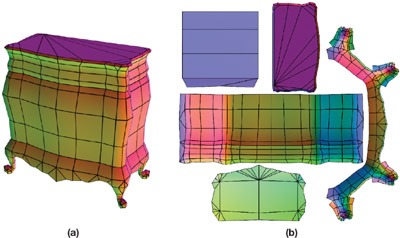
Figure 22-1 A Sample Model
The next step is to trace a ray from the interpolated boundary cage position in the direction of the reference model. This may result in more than one hit along the direction of the ray, and from each hit we will derive a candidate normal. We then select the most appropriate normal, which in our case will be the closest to the boundary cage.
22.1.2 The Boundary Cage
The boundary cage (or projection cage) usually consists of a mesh extruded from the working model. The artist may visually modify the cage to provide finer control over the way the rays are cast and to avoid complications in certain regions of the mesh.
The cage surface will serve as a starting point for the rays being cast onto the reference model. The vector from each vertex in the cage to the matching vertex on the working model is also interpolated during rasterization and used as the ray direction.
Usually the cage is built so that it encloses both the reference model and the working model. As you can see from the sample in Figure 22-2, if a ray is cast as previously described, we can assume that the hit closest to the cage can be used to extract the normal for the current pixel.
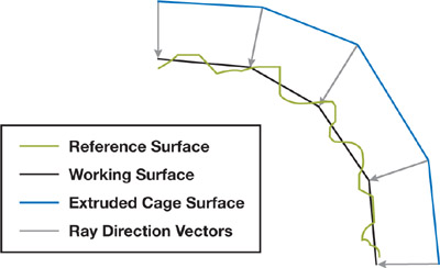
Figure 22-2 A Boundary Cage
22.2 Acceleration Structures
This implementation relies heavily on the ray tracing of high-polygon meshes, which can be extremely computational intensive without the use of proper acceleration structures. This is obviously also an issue when dealing with ray-tracing algorithms on the GPU (Purcell et al. 2002, Christen 2005). In this case, the choice of an acceleration structure is less trivial because we are dealing with an architecture designed for highly parallel vertex and fragment shading (Lindholm et al. 2001).
We need a structure that maps well to GPU memory using texture resources. We also need to take advantage of the fact that the working and reference meshes are mostly spatially coherent (in other words, they roughly share the same space).
22.2.1 The Uniform Grid
The uniform grid, as shown in Figure 22-3, is a spatial subdivision scheme that partitions the mesh into constant-size voxels or cells, as described in Fujimoto and Iwata 1985.
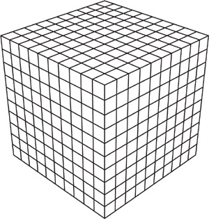
Figure 22-3 A Perspective View of a Uniform Grid
To date, most publications on GPU ray tracing use a uniform grid for spatial subdivision and 3D digital differential analyzer (3D-DDA) for grid traversal. The structure maps well to GPU memory and the traversal algorithm is simple enough to be implemented in a pixel shader.
For general-purpose ray-tracing computations, the uniform grid may not be the best option (Havran 2001). In our specific case, however, it is a very good candidate. As you can see in Figure 22-4, where the grid overlays both models, the working model's surface is always very close to that of the reference model. This coherence can be exploited efficiently using a 3D-DDA traversal algorithm.
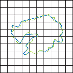
Figure 22-4 Both Models and the Grid Overlaid
22.2.2 The 3D Digital Differential Analyzer
First introduced by Amanatides and Woo 1987, the 3D-DDA algorithm allows a fast voxel traversal between two voxels in a uniform grid.
The 3D-DDA algorithm requires only a small number of steps to correctly guide the ray as it travels between neighboring cells. The cost of traversal is linear to the number of voxels visited. In most cases, however, the path is very short, which reduces the average traversal cost. Also note that the voxels, and therefore the geometry, are visited in the correct order, meaning that a valid hit will occlude any hits in the remaining cells. Figure 22-5 illustrates this approach.
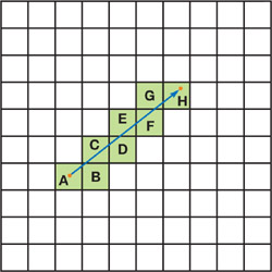
Figure 22-5 A Ray Traversing Grid Cells Using 3D-DDA
This algorithm, along with the uniform grid scheme, is a key component in exploring the spatial coherency between the meshes involved in the projection.
22.3 Feeding the GPU
Mapping the uniform grid and reference geometry data to hardware has been presented almost the same way in most publications about GPU ray tracing. The data structure used in this chapter is mostly based on previous publications on GPU ray tracing, with the exception of using indexed triangle lists to save video memory. See Figure 22-6 for a representation of the data structure.
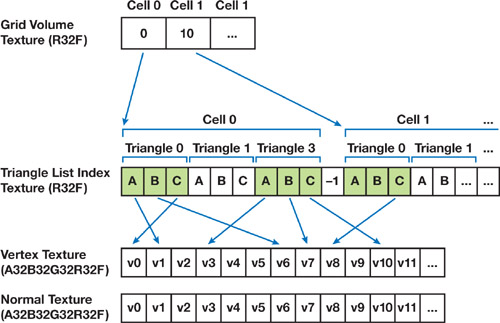
Figure 22-6 A Visual Representation of Data Mapped to the GPU
The uniform grid is stored as a 3D texture with the same size. Each voxel contains a pointer to the triangle list of the respective grid cell. Addressing the uniform grid consists simply of using normalized cubic coordinates when fetching data from the 3D texture. We will be referring to cubic coordinates as values between zero and the size of the grid. Helper functions to convert between grid coordinates are shown in Listing 22-1.
The triangle lists for each cell are stored in a separate 2D texture. Each entry on the triangle list contains a triplet of pointers to the respective triangle vertices in the geometry textures. The list is terminated by a null pointer. If the first pointer is null, it means the cell is empty. Addressing the 2D textures as a linear array requires a simple conversion, as you can see in Listing 22-2.
Example 22-1. Helper Functions That Convert Between Grid Coordinates
float3 CoordCubicToSpatial(float3 cubic)
{
  float3 normCubic = cubic * g_invGridCubicSize;
  return g_gridSpatialMinPoint + (normCubic * g_gridSpatialSize);
}
float3 CoordSpatialToCubicNorm(float3 spatial)
{
  return (spatial - g_gridSpatialMinPoint) * g_invGridSpatialSize;
}
Example 22-2. A Function That Maps a Linear Array Coordinate to a 2D Texture Coordinate
float2 Coord1Dto2D(float index, float2 invTexSize)
{
  float offset = index * invTexSize.x;
  float x = frac(offset);
  float y = (offset - x) * invTexSize.y;
  return float2(x, y);
}
The reference mesh is stored as a set of 2D textures. We keep the vertex positions and the normals separated because they won't need full 32-bit precision.
22.3.1 Indexing Limitations
For simplification purposes, we use 32-bit float indices, which provide us with an effective indexing range of 24 bits. This is probably enough because we are using only one texture for each data type and dealing with graphics cards that have a maximum texture size of 4,096.
To build a robust implementation and support reference meshes with millions of triangles, we could go beyond 24-bit indexing by using a packed 32-bit (RGBA) integer format. This way we could store the mesh across a maximum of 256 textures, using one of the packed elements to index the texture and the remaining element to index the data within the texture. However, directly addressing multiple textures in DirectX 9.0 class cards might involve emulating texture arrays with a 3D texture. This type of addressing could also be used on pointers stored in the grid texture.
22.3.2 Memory and Architectural Limitations
The base hardware specification used to test the solution presented in this chapter consisted of a Shader Model 3.0 medium-range ATI graphics card with 256 MB. This specific card is limited to power-of-two volumes, so the highest resolution volume we can safely allocate on this card is 256x256x256. However, when working with dense reference meshes with millions of polygons, we need to use a higher-resolution uniform grid to reduce the cost of visiting a cell containing geometry. Some NVIDIA cards already support non-power-of-two volumes.
Table 22-1 provides the memory usage statistics for a sample reference mesh with 700,000 triangles. Note that all textures used are power-of-two.
Table 22-1. Memory Usage Statistics for a Sample Reference Mesh
|
Description |
Dimensions |
Format |
Size |
|
Grid Texture |
256x256x256 |
R32F |
64 MB |
|
Triangle List Texture |
4096x2048 |
R32F |
32 MB |
|
Vertex Texture |
1024x1024 |
A32B32G32R32F |
8 MB |
|
Normal Texture |
1024x1024 |
A16B16G16R16F |
4 MB |
|
Total Size: |
108 MB |
Although the vertex and normal textures consume only a small portion of the memory footprint required, they can be packed tighter, trading off accuracy for memory. The vertex texture could be reduced by half by using a 16-bit floating-point texture format (for example, A16B16G16R16F), which would be precise enough for some models. The normals could also be stored in a low-precision texture using a 32-bit packed format such as A8R8G8B8, which would also halve the memory costs.
22.4 Implementation
In this chapter we analyze only a basic implementation of the typical projection using the pixel shader. This version requires only a single rendering pass of the working model. It has, however, a few limitations related to static flow control on Shader Model 3.0 hardware, where the maximum number of iterations for each loop must not exceed 256.
Later we discuss possible workarounds for this limitation, including an implementation that involves multipass and tiled rendering. And at the end of this section, we cover antialiasing.
22.4.1 Setup and Preprocessing
The first step in implementing the projection is to load both meshes and generate a uniform grid based on the high-polygon reference model. The grid and geometry data are then mapped to textures in video memory so they can be used by the pixel shader.
The working model, however, should be mapped to hardware vertex buffers and include a tangent basis, which will be used to transform the world-space normal (extracted from the reference model) into tangent space. A cage position and a texture coordinate set for each vertex are also required.
Texture samplers—which include the grid volume, the triangle list, and the geometry textures—must be set before rendering. Sampling filters must be disabled because we are using integer indexing. Clamp addressing should also be set.
Listing 22-3 shows a few common data structures declared in the beginning of the shader. These define a grid cell, an axial-aligned bounding box, a ray, and a triangle. Also listed are a few utility functions to access the grid cells, and a few to access geometry texture data.
Please note that the functions RayAABBIntersect() and RayTriangleIntersect() are not included in the listing, but they can be found in the complete shader provided on this book's accompanying DVD.
Example 22-3. Common Data Structures
struct Cell
{
  float3 cubicNormPos;
  // Current cubic position in the grid
  float3 cubicPos;
  // Current spatial position in the grid
  float triListStartIndex;
  // Pointer to the start of the tri-list
};
struct AABB
{
  float3 center;
  float3 extents;
};
struct Ray
{
  float3 origin;
  float3 dir;
};
struct Triangle
{
  float3 p0;
  float3 p1;
  float3 p2;
};
bool GetCellAtPoint(out Cell cell, in float3 spatialPos)
{
  // Convert spatial to normalized cubic coordinates.
  cell.cubicNormPos = CoordSpatialToCubicNorm(spatialPos);
  // Compute unnormalized cubic coordinates.
  cell.cubicPos = cell.cubicNormPos * g_gridCubicSize;
  // Fetch the grid volume texture and find the pointer to the
  // beginning of this cell's triangle list.
  const float4 coord = float4(cell.cubicNormPos, 0);
  cell.triListStartIndex = tex3Dlod(gridSampler, coord).r;
  // Check if we are inside the grid.
  return (cell.cubicNormPos > = 0) & &(cell.cubicNormPos < = 1);
}
float3 GetCellMinPoint(in Cell cell)
{
  return g_gridSpatialMinPoint + int3(cell.cubicPos) * g_cellSpatialSize;
}
float3 GetCellMaxPoint(in Cell cell)
{
  return g_gridSpatialMinPoint + (int3(cell.cubicPos) + 1) * g_cellSpatialSize;
}
float GetTriangleListIndex(float index)
{
  float4 tc = float4(Coord1Dto2D(index, g_invIndexTexSize), 0, 0);
  return tex2Dlod(indexSampler, tc).x;
}
float3 GetVertex(float index)
{
  float4 tc = float4(Coord1Dto2D(index, g_invVertexTexSize), 0, 0);
  return tex2Dlod(vertexSampler, tc).xyz;
}
float3 GetNormal(float index)
{
  float4 tc = float4(Coord1Dto2D(index, g_invNormalTexSize), 0, 0);
  return tex2Dlod(normalSampler, tc).xyz;
}
22.4.2 The Single-Pass Implementation
In this version of the algorithm, we render the working model directly to the normal-map render target only once. Following is a description of the steps taken inside the pixel shader.
Step 1
As shown in Listing 22-4, we start by using the interpolated vertex position and cage vector, both sent by the vertex shader, to set up the ray for the current pixel. We may need to adjust the origin of the ray if the cage falls outside the grid, as shown in Figure 22-7. We do this by intersecting the ray with the uniform grid's box to compute the first position along the ray that falls inside the grid. We use the adjusted origin of the ray to find the cell where we will begin the traversal.
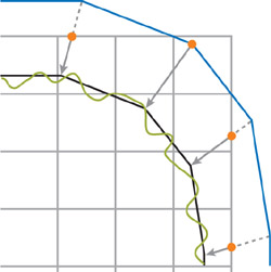
Figure 22-7 The Cage May Fall Outside the Grid at Some Points
Example 22-4. Setting Up the Ray
// Set up the ray using interpolated position and cage vector.
Ray ray;
ray.dir = -Input.cageDir.xyz;
ray.origin = Input.position + Input.cageDir.xyz;
// Check if we are currently outside the grid.
Cell cell;
if (GetCellAtPoint(cell, ray.origin))
{ // Compute the grid's min and max points.
  const float3 gridMin = g_gridSpatialMinPoint;
  const float3 gridMax = g_gridSpatialMinPoint + g_gridSpatialSize;
  // Compute intersection between the grid and the ray to find a
  // starting point within the boundaries of the grid.
  float t = 0;
  RayAABBIntersect(ray, gridMin, gridMax, t);
  // Adjust the ray origin to start inside the grid.
  ray.origin += ray.dir * t;
  // Find the first cell to begin traversal.
  GetCellAtPoint(cell, ray.origin);
}
Step 2
The next step is to compute the vectors step, tmax, and delta, as described in Amanatides and Woo 1987, where step indicates whether the current position should be incremented or decremented as the ray crosses voxel boundaries. The vector tmax stores the value of t at which the ray crosses the voxel boundary in each axis. Delta indicates how far along the ray we must move (in units of t) along each direction to match the dimensions of the voxel. Listing 22-5 shows how to initialize step, tmax, and delta.
Example 22-5. Preparing for 3D-DDA
// Compute tmax
float3 cellMin = GetCellMinPoint(cell);
float3 cellMax = GetCellMaxPoint(cell);
float3 tmaxNeg = (cellMin - ray.origin) / ray.dir;
float3 tmaxPos = (cellMax - ray.origin) / ray.dir;
float3 tmax =
    (ray.dir < 0) ? tmaxNeg : tmaxPos; // Compute traversal steps based on
// ray direction and cell dimensions.
float3 step = (ray.dir < 0) ? float3(-1, -1, -1) : float3(1, 1, 1);
float3 tdelta = abs(g_cellSpatialSize / ray.dir);
Step 3
We are now ready to begin traversing the grid. As you can see, the traversal code requires only a few instructions, which can be further optimized using vectorized static branching. The main loop is used to traverse the grid to the next cell, while the nested secondary loop is used to test the ray against all triangles in the current cell. See Listings 22-6 and 22-7.
Example 22-6. The Function Containing the Secondary Loop
This function checks all triangles in the cell and returns the normal closest to the ray origin (in the cage).
float3 FindNormalAtCell(in Cell cell, in Ray ray)
{
  // Prepare temporary vars:
  // - last_indices holds the vertex indices for the winning triangle
  // - last_ret holds the barycentric coords for the winning normal
  float3 indices, ret;
  float3 last_indices = 0;
  float3 last_ret = float3(0, 0, FLT_MAX);
  // Get the first vertex index; might be a terminator index (-1).
  float index = cell.triListStartIndex;
  float nextIndex = GetTriangleIndex(index++);
  // Loop until we find a terminator index.
  while (nextIndex > = 0)
  {
    // Get remaining vertex indices.
    indices.x = nextIndex;
    indices.y = GetTriangleListIndex(index++);
    indices.z = GetTriangleListIndex(index++);
    // Get triangle vertex positions.
    tri.p0 = GetVertex(indices.x);
    tri.p1 = GetVertex(indices.y);
    tri.p2 = GetVertex(indices.z);
    if (RayTriangleIntersect(ray, tri, ret) > 0)
    {
      // Use the current hit if closer to the ray origin.
      bool closest = (ret.z < last_ret.z);
      last_indices = closest ? indices : last_indices;
      last_ret = closest ? ret : last_ret;
    }
    // Get next index; might be a terminator index (-1).
    nextIndex = GetTriangleListIndex(index++);
  }
  // Check if we have a valid normal.
  float3 normal = 0;
  if (last_indices.x * last_indices.y > 0)
  {
    // Get normals from the winning triangle.
    float3 n0 = GetNormal(last_indices.x);
    float3 n1 = GetNormal(last_indices.y);
    float3 n2 = GetNormal(last_indices.z);
    // Interpolate normal using barycentric coordinates.
    float u = last_ret.x;
    float v = last_ret.y;
    float t = 1 - (u + v);
    normal = n0 * t + n1 * u + n2 * v;
  }
  return normal;
}
Example 22-7. The Main Loop in the Pixel Shader
Traversing the grid searching for a valid normal.
float3 normal = 0;
float done = 0;
while (!done)
{
  // Find a valid normal in the current cell.
  normal = FindNormalAtCell(cell, ray);
  // Advance to the next cell along the ray using 3D-DDA.
  float3 nextCubicPos = cell.cubicPos;
  if (tmax.x < tmax.y)
  {
    if (tmax.x < tmax.z)
    {
      nextCubicPos.x += step.x;
      tmax.x += tdelta.x;
    }
    else
    {
      nextCubicPos.z += step.z;
      tmax.z += tdelta.z;
    }
  }
  else
  {
    if (tmax.y < tmax.z)
    {
      nextCubicPos.y += step.y;
      tmax.y += tdelta.y;
    }
    else
    {
      nextCubicPos.z += step.z;
      tmax.z += tdelta.z;
    }
  }
  // Get the cell at the current point.
  bool insideGrid = GetCellAtCubicPos(cell, nextCubicPos);
  // We are done traversing when:
  // - We found a valid normal. Success.
  // - We fell outside the grid. Failure.
  done = (dot(normal, normal) > 0) || !insideGrid;
}
Step 4
To complete the pixel shader, we just need to convert the normal into the working model's tangent space and scale it to the 0..255 range to be stored in a bitmap, as shown in Listing 22-8.
Example 22-8. Converting the Normal to Tangent Space
float3 normalTS;
normalTS.x = dot(normal, Input.binormal);
normalTS.y = dot(normal, Input.tangent);
normalTS.z = dot(normal, Input.normal);
normalTS = normalize(normalTS);
return float4(normalTS * 0.5 + 0.5, 1);
Limitation
As we discussed earlier, these loops in ps_3_0 are limited to 256 iterations. A possible workaround is to use two nested loops instead of a single loop, as shown in Listing 22-9, to theoretically achieve a total of 65,536 iterations for each nested pair. The DirectX 9.0 documentation does not address this specific case, though it does mention that the maximum nested loop depth is 4 and the maximum number of instructions executed by a pixel shader must be at least 65,536. This limit can be reached quite easily with a sufficiently complex reference model and a denser grid. You might have to revert to a multipass approach (described in Section 22.4.3) if the host GPU has such instruction limits.
Example 22-9. An Example of Using Two Nested Loops to Work Around the Limitation
// Nested pair for the main loop
while (!done)
{
  while (!done)
  {
    ...
        // Nested pair inside the FindNormalAtCell function
        while (nextIndex > = 0)
    {
      while (nextIndex > = 0)
      {
        ...
      }
    }
    ...
  }
}
22.4.3 The Multipass Implementation
To avoid having four nested loops inside the pixel shader, we could move some work to the CPU and perform the projection in multiple passes. To achieve this, we would need to split the pixel shader.
- The first pass would perform the same computations as described in the single-pass implementation (steps 1 and 2). Then we would store packed information about the cell and the ray, and store the variables step, tmax, and delta on a render texture to be accessed during the following traversal passes.
- The second pass and the next N passes would perform a single traversal step along the grid at each pixel. To avoid processing empty areas, this pass could use queries to track the rendered pixels and the stencil buffer.
- The last pass would convert all the pixels in the normal map to tangent space.
Limitation
The single and most obvious limitation of this implementation is the memory requirement to store all the temporary variables in texture memory; however, tiled rendering solves this problem.
Tiled Rendering
As described in Purcell et al. 2002, the memory requirement limitation can be overcome by splitting the rendering into pieces or tiles. One tile would be rendered at a time and copied to a texture in system memory, allowing the render textures to be reused. The size of the tiles could be defined according to the available resources.
22.4.4 Antialiasing
The technique presented in this chapter can be extended to support antialiasing in at least two ways:
- Expanding the pixel shader to trace more rays, each one with a different path deviation. The results would be used as samples to compute an alias-free normal.
- Rendering the normal map multiple times and jittering the working model's vertex and cage position each time. The samples would then be weighted and accumulated in the render target. The cost of using this method is linear with the number of passes. If a normal map takes around 1 second to render, a 16-sample antialiased normal map will take about 16 seconds.
22.5 Results
The reference model for our test sample has around 560,000 triangles. The working model, on the other hand, has only 868 triangles. Figures 22-8 and 22-9 show the models.
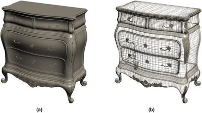
Figure 22-8 The Reference Model
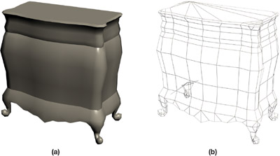
Figure 22-9 The Working Model
Preparing the reference model for projection takes only 5.2 seconds: 3.6 seconds to load the file, 1.0 second to generate the uniform grid, and 0.6 seconds to feed the data to the GPU. Please keep in mind that the CPU part of the implementation is not yet fully optimized and is using only a single core.
These timings were recorded on a notebook with a T2400 Core Duo processor, 1 GB DDR2 memory at 667 MHz, and a 5400 rpm hard drive. The graphics processor is an ATI X1600 with 256 MB of dedicated video memory.
The charts in Figure 22-10 compare the GPU implementation described in this chapter with two popular CPU-based implementations, NVIDIA Melody and xNormal. The boundary cage used is similar in all tests and the settings are the simplest possible, with no antialiasing, padding, or dilation.
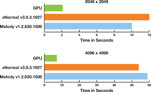
Figure 22-10 Performance Comparison Charts
The resulting normal map shows minor precision issues that can be solved by improving the numerical robustness of the algorithm in the pixel shader. See Figure 22-11.
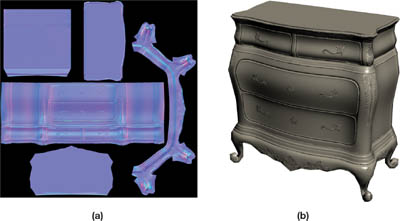
Figure 22-11 Resultant Normal Map and Its Application
The normal map was rendered against a black background for illustration purposes only. Creating the map against a midblue background (rather than black) will ameliorate mipmapping issues.
Possible Improvements
The reference mesh could be stored using triangle strips instead of lists: this would save texture memory by storing fewer triangle indices. It would also improve the performance in the pixel processor by reducing texture fetches.
The preprocessing part of this implementation, which runs on the CPU, could be optimized by using Streaming SIMD Extensions and OpenMP.
22.6 Conclusion
With minor modifications, this technique could be used to generate displacement maps, which can also be used for parallax and relief mapping. With a more complex shader, we could also generate local ambient occlusion or cavity maps.
One advantage of this technique is that it's fast enough to permit (and encourage) individually rendering all the mip levels explicitly, improving shading quality in mipmapped areas.
Because of the nature of the computations required for this technique, it scales very well with multithread-based architectures, which the latest generation of GPUs features.
In this chapter we have shown that the graphics processor can generate normal maps very efficiently, which allows fast, high-resolution previews.
22.7 References
Amanatides, John, and Andrew Woo. 1987. "A Fast Voxel Traversal Algorithm for Ray-tracing." In Proceedings of Eurographics '87, pp. 3–10. Available online at http://www.cse.yorku.ca/~amana/research/.
Christen, Martin. 2005. "Ray Tracing on GPU." University of Applied Sciences Basel, diploma thesis. Available online at http://www.clockworkcoders.com/oglsl/rt/.
Cohen, Jonathan, Marc Olano, and Dinesh Manocha. 1998. "Appearance-Preserving Simplification." In Proceedings of the 25th Annual Conference on Computer Graphics and Interactive Techniques, pp. 115–122. Available online at http://www.cs.unc.edu/~geom/APS/.
Fujimoto, A., and K. Iwata. 1985. "Accelerated Ray Tracing." In Computer Graphics: Visual Technology and Art (Proceedings of Computer Graphics, Tokyo '85), pp. 41–65.
Havran, Vlastimil. 2001. "Heuristic Ray Shooting Algorithms." Czech Technical University, Ph.D. dissertation. Available online at http://www.cgg.cvut.cz/~havran/phdthesis.html.
Heidrich, Wolfgang, and Hans-Peter Seidel. 1999. "Realistic, Hardware-accelerated Shading and Lighting." In Proceedings of SIGGRAPH 99, pp. 171–178. Available online at http://www.cs.ubc.ca/~heidrich/Papers/Siggraph.99.pdf.
Krishnamurthy, Venkat, and Marc Levoy. 1996. "Fitting Smooth Surfaces to Dense Polygon Meshes." In Proceedings of the 23rd Annual Conference on Computer Graphics and Interactive Techniques, pp. 313–324. Available online at http://graphics.stanford.edu/papers/surfacefitting/.
Lindholm, Erik, Mark Kilgard, and Henry Moreton. 2001. "A User Programmable Vertex Engine." Presentation at SIGGRAPH 2001. Available online at http://developer.nvidia.com/object/SIGGRAPH_2001.html.
Purcell, Timothy J., Ian Buck, William R. Mark, and Pat Hanrahan. 2002. "Ray Tracing on Programmable Graphics Hardware." In ACM Transactions on Graphics (Proceedings of SIGGRAPH 2002) 21(3), pp. 703–712. Available online at http://graphics.stanford.edu/papers/rtongfx/.
- Contributors
- Foreword
- Part I: Geometry
-
- Chapter 1. Generating Complex Procedural Terrains Using the GPU
- Chapter 2. Animated Crowd Rendering
- Chapter 3. DirectX 10 Blend Shapes: Breaking the Limits
- Chapter 4. Next-Generation SpeedTree Rendering
- Chapter 5. Generic Adaptive Mesh Refinement
- Chapter 6. GPU-Generated Procedural Wind Animations for Trees
- Chapter 7. Point-Based Visualization of Metaballs on a GPU
- Part II: Light and Shadows
-
- Chapter 8. Summed-Area Variance Shadow Maps
- Chapter 9. Interactive Cinematic Relighting with Global Illumination
- Chapter 10. Parallel-Split Shadow Maps on Programmable GPUs
- Chapter 11. Efficient and Robust Shadow Volumes Using Hierarchical Occlusion Culling and Geometry Shaders
- Chapter 12. High-Quality Ambient Occlusion
- Chapter 13. Volumetric Light Scattering as a Post-Process
- Part III: Rendering
-
- Chapter 14. Advanced Techniques for Realistic Real-Time Skin Rendering
- Chapter 15. Playable Universal Capture
- Chapter 16. Vegetation Procedural Animation and Shading in Crysis
- Chapter 17. Robust Multiple Specular Reflections and Refractions
- Chapter 18. Relaxed Cone Stepping for Relief Mapping
- Chapter 19. Deferred Shading in Tabula Rasa
- Chapter 20. GPU-Based Importance Sampling
- Part IV: Image Effects
-
- Chapter 21. True Impostors
- Chapter 22. Baking Normal Maps on the GPU
- Chapter 23. High-Speed, Off-Screen Particles
- Chapter 24. The Importance of Being Linear
- Chapter 25. Rendering Vector Art on the GPU
- Chapter 26. Object Detection by Color: Using the GPU for Real-Time Video Image Processing
- Chapter 27. Motion Blur as a Post-Processing Effect
- Chapter 28. Practical Post-Process Depth of Field
- Part V: Physics Simulation
-
- Chapter 29. Real-Time Rigid Body Simulation on GPUs
- Chapter 30. Real-Time Simulation and Rendering of 3D Fluids
- Chapter 31. Fast N-Body Simulation with CUDA
- Chapter 32. Broad-Phase Collision Detection with CUDA
- Chapter 33. LCP Algorithms for Collision Detection Using CUDA
- Chapter 34. Signed Distance Fields Using Single-Pass GPU Scan Conversion of Tetrahedra
- Chapter 35. Fast Virus Signature Matching on the GPU
- Part VI: GPU Computing
-
- Chapter 36. AES Encryption and Decryption on the GPU
- Chapter 37. Efficient Random Number Generation and Application Using CUDA
- Chapter 38. Imaging Earth's Subsurface Using CUDA
- Chapter 39. Parallel Prefix Sum (Scan) with CUDA
- Chapter 40. Incremental Computation of the Gaussian
- Chapter 41. Using the Geometry Shader for Compact and Variable-Length GPU Feedback
- Preface